1.3.11. Materials and properties
These properties define both the material parameters and the sections, shells, solids, membranes and cables parameters.
In order to activate each material element, the user must select the element type in:
General data > Analysis > Element type.
1.3.11.1. Beams
1.3.11.1.1. Rectangular section
Materials and properties > Beams > Rectangular section
This condition is assigned to beams with its transversal section rectangular.
Fig. 1.26 Window for defining a beam of rectangular section.
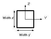
Fig. 1.27 Frame of references for beams.
The Width y is the width of the rectangular section following the Y’ direction. Width z is the width in the Z’ direction. G is the torsion modulus and E is the Young modulus.
Note: Remember that for an isotropic material:
The Specific Weight (different from density). The weight is considered in the direction of the gravity, which will be defined later. Its default units are \(N/m^3\). Once the values are filled in, the condition must be assigned to the beams.
1.3.11.1.2. Generic section
Materials and properties > Beams > Generic section
The definition of the properties for a general beam section is very similar to that of the rectangular section. Instead of giving the width and height of the section, the area (A), the Torque modulus (J) and the inertia modulus for the Y’ (Inertia y) and Z’ axes (Inertia z) of the beam are given. Default units for the area are \(m^2\) and for the inertia modulus are \(m^4\).
It is also possible to automatically calculate the properties of predefined sections (Rectangular Solid, Trapezoidal Solid, Circular Solid, SemiCircular Solid, Tube , Double T), inserting the desired dimensions in the window which pops-up after pressing the “Predefined Sections” button.
1.3.11.1.3. Sections library
Materials and properties > Beams > Sections library
There is a wide library available in RamSeries for defining standard steel sections, suitable for any engineering discipline, such as civil, or naval. By this means, RamSeries provides a database of beam sections for the users, helping them to reduce time defining materials.
This windows allows to edit the type of beam section and its material. In addition, the position of the center related to its natural position, named Z axe, can be redefined. This feature allows to determine the second moment of area of the beam about any parallel axis through its neutral axis.
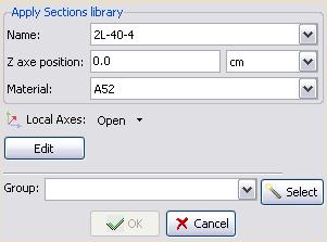
Fig. 1.28 Section library window.
If the button Edit is pressed, the sections library window is displayed, and it is possible to choose the desired section and check the geometrical properties.
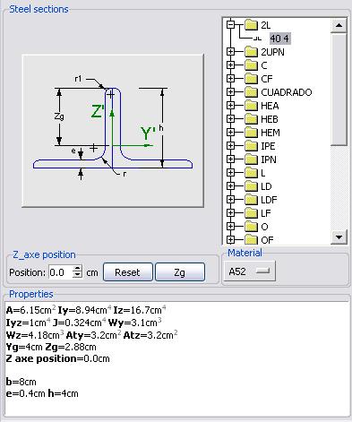
Fig. 1.29 Edition window.
1.3.11.1.4. Naval stiffeners
In RamSeries, it is possible to assign properties of fiber reinforced plastic stiffeners to beams, named \(\omega\) section. Composite \(\omega\) beams are made of a core material (such as PVC) covered by fibre reinforced plastic (FRP), which gives its strength and stiffness. These kind of profiles are very common in naval motorcraft or sailing composite hulls.
Materials and properties > Beams > Naval stiffeners
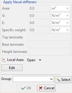
Fig. 1.30 Naval stiffeners window selection.
After pressing the button Edit, the following window will show up:
FIGURE
In the Edit window, the user can edit the geometrical properties of the naval stiffeners, and select the materials of which it is made of, it is the laminate. Besides, the shear modulus of the core material is defined in this window.
Different materials can be selected for the top, bottom and sides of the stiffener, allowing to define a very specific composite profile. In addition, this window enables to show the geometrical properties of the stiffener.
The materials that can be used to define naval stiffeners are those defined as classic constitutive model (obtained by classical laminate theory). The list of laminates defined can be found in:
Materials and properties > Physical properties > Laminates.
For further information regarding the definition of Laminate materials, the user is referred to composite materials section of this manual.
1.3.11.2. Cables
Materials and properties > Cables
The main difference between cable and beam elements is that the cable section can be considered as zero in comparison with its length. As a consequence, the flexure stiffness of cables can be assumed as zero. Therefore, they are subjected only to normal stresses.
Cable materials are used for simulating elements such as mooring lines. The variables for defining cables are its section area and material properties (Young modulus and specific weight).
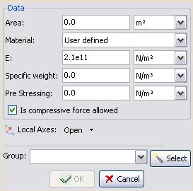
Fig. 1.31 Window for defining cable sections.
1.3.11.3. Damper
Materials and properties > Damper
1.3.11.3.1. Linear Damper
Materials and properties > Damper > Linear damper
They are only available for linear dynamic analyses.
They enable the application of stiffness and damping in the three global directions (x, y, and z) to a geometric line.
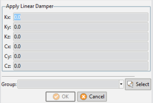
Fig. 1.32 Window for defining linear damper properties.
1.3.11.4. Shells
Materials and properties > Shells
Shells are used for simulating structures which one of its dimension is much smaller than the other two dimensions. Therefore, shells allow to predict the behaviour of 3D structures, but at much lower computational cost. Examples of their application are the hull of a ship, or the walls of a building.
All shells materials in RamSeries have two parameters in common that can be defined:
Material definition: This option allows to assign the shell with a physical material. See Physical properties section of this manual.
Local axes: RamSeries allows the definition of local axes in surfaces. How to assign local axes to the geometry is described in Global and local axes section of this manual.
For a deeper understanding of the formulation of shells, the user is referred to the RamSeries theory manual, section Analysis of shells.
New materials can be created in the Physical properties section of the data tree:
Materials and properties > Physical properties.
Shell materials are assigned to surfaces. To define a surface as a shell, open Shells and Select the surface to assign.
1.3.11.4.1. Isotropic shell
Materials and properties > Shells > Isotropic shells
The definition of an elastic shell requires the specification of material properties and the actual thickness of the shell. In the isotropic case, the specification of material properties simply consists on providing the Young’s modulus, the Poisson’s coefficient and the specific weight of the material. This can be done by either providing user defined values (as seen in the figure below) or selecting a pre-defined material from those available in the drop-down list. In addition, the actual thickness of the shell must be provided since this is not an intrinsic material’s parameter but a physical property of the structural element to which the shell is going to be applied.
Note that for an isotropic material the shear modulus is already given once the Young’s modulus and the Poisson coefficient have been specified:
Once all the required properties have been introduced, the shell’s definition can be assigned to the desired group of surface geometrical entities in the CAD model.
1.3.11.4.2. Orthotropic shell
Materials and properties > Shells > Orthotropic shells
Similarly to the isotropic case, orthotropic shell’s definition requires the user to provide the actual thickness of the shell and the properties of the constituent material. In the orthotropic case, material properties are specified by selecting a pre-defined orthotropic material from the drop-down list. The actual thickness of the shell must be provided since this is not an intrinsic material’s property but a geometrical parameter of the structural element to which the shell is going to be applied. In addition, the orthotropy axes must be defined using the Local axes option in the dialog box shown below. If local axes are not specified, the orthotropy axes are set by default to coincide will the global axes.
Typical applications of orthotropic shell materials are laminate materials.
The parameters to define for orthotropic materials are described in:
Materials and properties > Physical properties > Orthotropic
1.3.11.4.3. Laminate shell
Materials and properties > Shells > Laminate shells
As well as for the case of “Naval stiffeners”, it is possible to use in RamSeries laminated fiber reinforced polymer shells. To this aim, the user must simply select a pre-defined laminate material from the drop-down list and apply it to the desired group of surface geometrical entities in the CAD model.
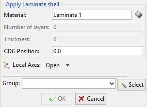
Fig. 1.33 Window for selecting laminate shell.
By clicking on the “Edit Laminate” button (at the right side of the material’s entry), a list of the available laminates is displayed in a separate window (as seen in the figure below) thus allowing the selection and the interactive edition of existing laminates, and even the creation of new ones.
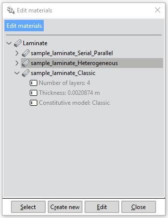
Fig. 1.34 Window for selecting the edition of a sample laminate material.
As stated above, during the definition of a laminated shell group a previously defined laminate material must be selected. RamSeries graphic user interface provides few sample laminates but new ones can be created in the following section of the data tree:
Materials and properties > Physical properties > Laminates.
Further description of how to define composite materials is found in Composites section of this manual.
1.3.11.4.4. Stiffened shell
Materials and properties > Shells > Stiffened shells
Some types of structures can be modelled as a shell reinforced with beams, such as the hull of a ship or metal civil structures. In these cases, the user must define each position of beams. Instead of it, in RamSeries it is possible to only assign a shell which will have the properties of a reinforced plate with stiffeners welded onto it. Consequently, the users have not to model all beams, saving time to them.
The window for assigning a stiffened shell is the following:
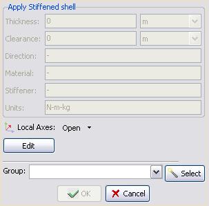
Fig. 1.35 Window for assigning stiffened shells.
For defining the properties of this plate, the user must select Edit button. By selecting it, the following data can be defined:
Thickness: thickness of the shell.
Clearance: distance between stiffeners.
Stiffener direction: direction in which stiffeners are encountered.
Stiffener section: the type of reinforcement section used for reinforcing the shell. All the profile sections found in Sections library section are also available in this option.
Stiffener material: three types of steel materials can be used, A37, A42 or A52.
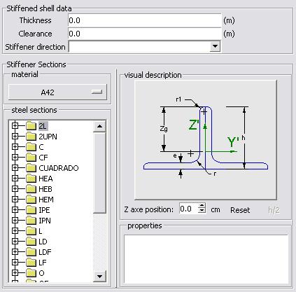
Fig. 1.36 Window for defining stiffened shell properties.
1.3.11.4.5. Plasticity shell
Materials and properties > Shells > Plasticity shells
This option is used for defining a material with plasticity constitutive model. The properties of these materials can be found in:
Materials and properties > Physical properties > Plasticity.
1.3.11.5. Membranes
Materials and properties > Membranes
Membranes are used for simulating fabric-like objects and structures, which do not support or transmit moment loads. In the case of compression loads, membrane materials tend to wrinkle. Applications of membranes are tents, airbags, or parachutes.
The following parameters can be defined for membranes:
Thickness: thickness of the membrane.
Material: membrane’s material. It can be defined isotropic membrane or orthotropic membrane. The difference between them is similar as the case of isotropic shell and orthotropic shell (see Damper). For isotropic membrane an isotropic material are used. On the other hand, for orthotropic membrane an orthotropic material are used.
Consider wrinckling: a membrane does not resist compression loads, but it is wrinkled. When compression stress is higher than this limit, wrinkling algorithm, that manages the wrinking process, is activated.
Allowed compression stress (Pa): tolerance for activating the wrinkling algorithm. If compression stress is higher than the tolerance.
Pre-stress: Membrane pre-stressing. In local axes.
Local axes: defined in Global and local axes.
1.3.11.6. Solids
Materials and properties > Solids
Solids allow to predict the behaviour of 3D structures, which require a high level of detail. However, it must bear in mind that the simulation is conducted at higher computational cost than Shells. The main reason is that solids require a higher mesh discretization of the geometry, hence, more finite elements are generated. Examples of their application are joint or structural details, or impacts between objects.
In order to assign Solids, the user must activate solid elements in:
General data > Analysis > Element types > solids.
Solid materials are assigned to volumes. To define a volume as a solid, open Solids and Select the volume to assign.
For a deeper understanding of the formulation of solids, the user is referred to the RamSeries theory manual, section Analysis of three-dimensional solids.
New materials can be created in the Physical properties section of the data tree:
Materials and properties > Physical properties.
1.3.11.6.1. Isotropic solids
Materials and properties > Solids > Isotropic solid
This condition is assigned to solid volumes. Properties to enter are:
Material. To be chosen from library, or “User defined”.
E is the Young modulus (\(2.1e^{11} N/m^2\) for steel) and ν is the Poisson coefficient with value 0.3 for steel (it is non-dimensional).
Specific Weight is the self-weight of the solid (different from density). The weight is considered in the direction of the gravity, which will be defined later. Its default units are \(N/m^3\).
Once the values are filled in, the condition must be assigned to the volume that defines the solid.
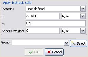
Fig. 1.37 Window for defining isotropic solids.
1.3.11.6.2. Orthotropic solids
Materials and properties > Solids > Orthotropic solid
Properties defined in this condition are similar to that of the Isotropic solid condition. The difference is that the material is orthotropic. The orthotropy axes are the ones defined in the Global and local axes section. The properties to enter are the Young Modulus (\(E_x\), \(E_y\)), the Poisson coefficients (\(ν_{xy}\), \(ν_{yx}\)) and the Shear modulus (\(G_{xy}\), \(G_{xz}\), \(G_{yz}\)). They are all referred to the local axes X’ and Y’.
1.3.11.6.3. Plasticity solid
Materials and properties > Solids > Plasticity solid
Assigns solids with plasticity constitutive model to volumes.
This material is similar than plasticity on shells. Instead of applying it to surfaces, it is applied to volumes.
1.3.11.6.4. Laminate solid
Materials and properties > Solids > Laminate solid
Assigns composite solids to volumes. The model used to simulate the composite behaviour is the Serial/Parallel mixing theory. It is recommended to review the theory and reference manual referred to this model.
This material is similar than laminate shells. Instead of applying it to surfaces, it is applied to volumes.
1.3.11.7. Physical properties
Materials and properties > Physical properties
There is a wide library of materials available to choose in RamSeries.
The properties of these materials can also be edited and new materials can be created. These materials are the ones which can be chosen in the different Beams , Cables, Damper , Membranes , Solids Properties windows.
Material properties are grouped into various tabs according to their use and relevance for the various constitutive models available in RamSeries: Structural, Damage and Allowable stresses.
If the user selects Physical properties tab, the materials library is shown, grouping the materials in the following classification:
Steel: a library of steel alloys. They can assigned to any type of element (beam, shell, solid).
Concrete: a library of concrete. They can assigned to any type of element (beam, shell, solid).
Solid: a library of the most used metals, decomposed in titanium, stainless steel, aluminium and bronze alloys. They can assigned to any type of element (beam, shell, solid).
Plasticity: a library of materials assigned with plasticity.
Orthotropic: a library of orthotropic materials. See Orthotropic materials.
FRP reinforcement: a library of fibre materials for defining composite materials. See Composites.
FRP matrix: a library of matrix materials for defining composite materials. See Composites.
Composite layer: in this section the user can create unidirectional plies by choosing its compoundings. The models used for simulating these materials are rule of mixtures or serial/parallel mixing theory. Classical laminate theory can not be used. See Composites.
Laminate: in this section the user can create composite laminates, which will be assigned to geometries. The user can choose which composite model: classical laminate theory, rule of mixtures or serial/parallel mixing theory. See Composites.
New materials can be created by right clicking on the desired material group.
1.3.11.7.1. Orthotropic materials
The properties required to define an orthotropic material are shown in the dialog box in the figure below. These consist on the longitudinal and transverse Young’s modulus (\(E_x\), \(E_y\)), the major Poisson’s ratio (\(ν_{xy}\)) and the shear modulus (\(G_{xy}\), \(G_{xz}\), \(G_{yz}\)). Note that all these properties are referred to the orthotropy axes of the material. The orientation of these material axes with respect to the global axes is given by the definition of the shell’s local axes.
Note
Remember that to maintain the elasticity hypothesis it is necessary to accomplish that:
Hence, only the major Poisson’s ratio needs to be specified since the minor Poisson’s ratio is internally evaluated in accordance to the relation above. Note than the transverse Young’s modulus \(E_z\) has no effect if this material is used to define an orthotropic shell. \(E_z\) is only taken into account when the orthotropic material is assigned to a solid. The same argument applies to Poisson’s coefficients different from the major Poisson’s ratio \(ν_{xy}\). Additional Poisson coefficients can be defined in the form of a 3x3 matrix (see the image below) but have only effect when the corresponding orthotropic material is assigned to a generic 3D solid.
Default units for \(E\) and \(G\) are \(N/m^2\) and \(ν\) is non-dimensional. Also note that for and orthotropic material the following relation should be satisfied.
Once all the required properties have been introduced, the shell’s definition can be assigned to the desired group of surface geometrical entities in the CAD model.
1.3.11.7.2. Elastic properties
Materials and properties > Material group > Structural properties > Elastic properties.
E: Young modulus.
G: Shear modulus.
\(\boldsymbol{\nu}\): Poisson coefficient.
Specific weight: weight per unit volume of the material.
Maximum stress: maximum acceptable stress for the material.
1.3.11.7.3. Plastic properties
Materials and properties > Plasticity > Plastic material > Structural > plasticity J2.
These properties are used for defining the plastic J2 constitutive model of the material.
The parameters are the following:
Tensile yield stress: Initial yield limit for the onset of plasticity.
Isotropic hardening: For isotropic hardening, the shape of the yield surface does not change during the deformation but its size increases with plastic deformation in accordance with the hardening law. Hence, the type of hardening law to be used must be specified for isotropic hardening. The available type are:
Linear: Linear (i.e. constant) hardening law. The constant ratio between the stress increment and the strain increment within the plastic regime must be provided.
Exponential: A power law is used to characterize the hardening of the material. A saturation stress must be provided together with the power law exponent.
Linear-Exponential: A combination of linear and exponential isotropic hardening is conducted.
Linear hardening: Slope of the linear hardening.
Saturation flow stress: Stress at which tends the material for high strain. If this value is lower than the yield stress, the material experiments a softening behaviour. On the contrary, if the saturation value is higher than yield stress, the material experiments a hardening behaviour.
Saturation hardening law exponent: Exponent for the exponential hardening/softening. Lower values of the exponent will lead to reach the saturation stress faster.
Kinematic hardening: For kinematic hardening, neither the shape not the size of the yield surface change during the deformation. But the yield surface is translated in the stress space. It allows for modelling non-symmetric tension/compression behaviors such for instance the Baushinger effect in metals.
Linear kinematic hardening:
1.3.11.7.4. Damage properties
The parameters in this section concern the non-linear isotropic damage model in RamSeries.
\(S_{yt}\): elastic threshold of the material.
Damage law: type of damage law to be used. It can be linear or exponential.
Linear
H/S Ratio: hardening/softening ratio
Exponential
\(G_f\): Fracture energy
\(S_{sat}\): Saturation stress.
Damage norm: damage norm to be used.
Symmetric Traction/Compression.
Traction.
Non-symmetric Traction/Compression.
C/T Ratio: Traction/compression ratio
1.3.11.7.5. Allowable stresses properties
the parameters in this section are used to evaluate failure criteria when the material under consideration is used in the definition of laminated composite materials.
\(S_{c1}\): allowable compression stress in direction 1.
\(S_{c2}\): allowable compression stress in direction 2.
\(S_{t1}\): allowable tension stress in direction 1.
\(S_{t2}\): allowable tension stress in direction 2.
\(T_{12}\): allowable shear stress (12).
\(T_{23}\): allowable shear stress (23).
\(T_{13}\): allowable shear stress (13).
1.3.11.8. Composites
Composite components: this set of parameters is only available for the definition of composite layers to be further used in the definition of laminated composite materials.
Fibre/Matrix Reinforcement material: reinforcement material to be used in the current composite ply Matrix material: matrix material to be used in the current composite ply Vf(%): volume content of fiber of the current composite ply
Monocomponent/core Ply material: monocomponent material to be used in the definition of a core ply
Laminates definition: in this section, laminated composites can be defined based on composite layers and/or orthotropic materials previously created within the materials’ library of RamSeries. To this aim, the laminate’s definition window shown in the following figure is provided to ease the creation of new laminated systems.
1.3.11.8.1. Composite calculator
A composite materials ‘calculator’ is provided in RamSeries to make easier the definition of composite material properties.
The properties of the composite’s components (fibre and resin) can be introduced separately in the calculator together with the volume fraction properties of the material. Based on these information and following the formulation in [NR546], the equivalent composite properties are evaluated, as well as the composite strengths to be used in the evaluation of the Tsai-Wu failure criteria.
By closing the calculator’s window, a new ‘composite layer’ orthotropic material is automatically created as well as the corresponding FRP reinforcement (Fibre) and FRP matrix (Resin) components.
1.3.11.9. Fatigue damage assessment
If Dynamic Analyses is activated, it is possible to perform a Damage Assessment based on the FEA stress results. (see Appendix 10: Fatigue Damage Assessment).
It is necessary to activate it in: General data > Analysis > Damage assessment.
Furthermore, predefined S-N curves may be inserted from a file, choosing
General data > Analysis > SN curves file.
Ask CompassIS for a sample file regarding this issue.
1.3.11.9.1. Shells damage assessment
By assigning this condition to any line of the geometry, the user is indicating the program that it is a welded connection, and that it must be verified for fatigue damage.
By assigning this condition to any surface of the geometry, the user is indicating the program that it must be verified for fatigue damage. The user can choose between the Standard Classification SN curves, or the Whöler curves.
INCLUDE two FIGURE (damage assessment for shells and for beams)
!!!!!!!!!**!!!!!!!!!
!!!!!!!!****!!!!!!!!
!!!!!!!******!!!!!!!
!!!!!!********!!!!!!
If predefined S-N curves have been inserted through a valid file as mentioned above, they will appear automatically by clicking on the SN curves button.
1.3.11.10. Laminate failure in materials
For shells:
Materials and properties > Shells > Failure in shells.
For solids:
Materials and properties > Solids > Failure in solids.