2.1.2.2. Analysis of three-dimensional solids

In this section, a summary of the theory of 3D solids analysis is provided. The basic assumptions under the formulation implemented within RamSeries are as follows:

1. Small displacements

2. Linear elasticity of materials

3. The principle of loads superposition

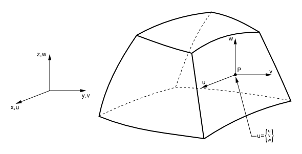
For a 3D solid, the displacement of a given point is completely determined by the values of the three degrees of freedom \(u, v, w\).

Fig. 2.3 Schematic representation of a 3D solid. The deformation of the solid is completely determined once the displacement field \((u,v,w)\) is known. Hence, three degrees of freedom must be considered for each material point.

Following the three-dimensional theory of elasticity, the deformation of the solid is defined, using the Voigt notation, as follows:

(2.20)\[\begin{split}\begin{aligned} \begin{bmatrix} \epsilon_x \\ \epsilon_y \\ \epsilon_z \\ \gamma_{xy} \\ \gamma_{xz} \\ \gamma_{yz} \\ \end{bmatrix} = \begin{bmatrix} \frac{\partial {u}}{\partial {x}} \\ \frac{\partial {v}}{\partial {y}} \\ \frac{\partial {w}}{\partial {z}} \\ \frac{\partial {u}}{\partial {y}} + \frac{\partial {v}}{\partial {x}} \\ \frac{\partial {u}}{\partial {z}} + \frac{\partial {w}}{\partial {x}} \\ \frac{\partial {v}}{\partial {z}} + \frac{\partial {w}}{\partial {y}} \\ \end{bmatrix} \end{aligned}\end{split}\]

In the most general case of anisotropic elasticity, the stress-strain relation is provided through a symmetric 6x6 constitutive matrix with 21 independent coefficients. Nevertheless, the more simple and commonly used orthotropic case is considered in RamSeries. Hence, considering \(x^{'},y^{'},z^{'}\) the principal orthotropic directions of the solid material, the constitutive equation in local axes can be written as:

(2.21)\[\begin{split}\begin{aligned} \begin{bmatrix} \epsilon^{'}_x \\ \epsilon^{'}_y \\ \epsilon^{'}_z \\ \gamma^{'}_{xy} \\ \gamma^{'}_{xz} \\ \gamma^{'}_{yz} \\ \end{bmatrix} = \begin{bmatrix} \frac{1}{E_{x^{'}}} & -\frac{\nu_{y^{'}x^{'}}}{E_{y^{'}}} & -\frac{\nu_{z^{'}x^{'}}}{E_{z^{'}}} & 0 & 0 & 0 \\ -\frac{\nu_{x^{'}y^{'}}}{E_{x^{'}}} & \frac{1}{E_{y^{'}}} & -\frac{\nu_{z^{'}y^{'}}}{E_{z^{'}}} & 0 & 0 & 0 \\ -\frac{\nu_{x^{'}z^{'}}}{E_{x^{'}}} & -\frac{\nu_{y^{'}z^{'}}}{E_{y^{'}}} & \frac{1}{E_{z^{'}}} & 0 & 0 & 0 \\ 0 & 0 & 0 & \frac{1}{G_{x^{'}y^{'}}} & 0 & 0 \\ 0 & 0 & 0 & 0 & \frac{1}{G_{x^{'}z^{'}}} & 0 \\ 0 & 0 & 0 & 0 & 0 & \frac{1}{G_{y^{'}z^{'}}} \\ \end{bmatrix} \begin{bmatrix} \sigma^{'}_x \\ \sigma^{'}_y \\ \sigma^{'}_z \\ \tau^{'}_{xy} \\ \tau^{'}_{xz} \\ \tau^{'}_{yz} \\ \end{bmatrix} \end{aligned}\end{split}\]

where only 9 independent material constants actually remain since the following relations must hold due to the symmetry of the constitutive matrix:

(2.22)\[\begin{aligned} E_{x^{'}}\nu_{y^{'}x^{'}} = E_{y^{'}}\nu_{x^{'}y^{'}} \ \ \ ; \ \ \ E_{y^{'}}\nu_{z^{'}y^{'}} = E_{z^{'}}\nu_{y^{'}z^{'}} \ \ \ ; \ \ \ E_{z^{'}}\nu_{x^{'}z^{'}} = E_{x^{'}}\nu_{z^{'}x^{'}} \end{aligned}\]

In the isotropic case only two material parameters, the Young’s modulus E and the Poisson coefficient ν, are required and the constitutive relation reduces to:

(2.23)\[\begin{split}\begin{aligned} \begin{bmatrix} \sigma_x \\ \sigma_y \\ \sigma_z \\ \tau_{xy} \\ \tau_{xz} \\ \tau_{yz} \\ \end{bmatrix} = \boldsymbol{D} \begin{bmatrix} \epsilon_x \\ \epsilon_y \\ \epsilon_z \\ \gamma_{xy} \\ \gamma_{xz} \\ \gamma_{yz} \\ \end{bmatrix} \end{aligned}\end{split}\]

where the stiffness matrix \(\boldsymbol{D}\) is given by:

(2.24)\[\begin{split}\begin{aligned} \boldsymbol{D} = \frac{E(1-\nu)}{(1+\nu)(1-2\nu)} \begin{bmatrix} 1 & \frac{\nu}{1-\nu} & \frac{\nu}{1-\nu} & 0 & 0 & 0 \\ & 1 & \frac{\nu}{1-\nu} & 0 & 0 & 0 \\ & & 1 & 0 & 0 & 0 \\ & & & \frac{1-2\nu}{2(1-\nu)} & 0 & 0 \\ & \it{Symm} & & & \frac{1-2\nu}{2(1-\nu)} & 0 \\ & & & & & \frac{1-2\nu}{2(1-\nu)} \\ \end{bmatrix} \end{aligned}\end{split}\]