2.1.2.1. Analysis of shells

Table 2.1 Glossary

Symbol	Description	SI units
\(x^{'} , y^{'} , z^{'}\)	Local shell coordinate directions	\(m\)
\(u^{'} , v^{'} , w^{'}\)	Displacements of a generic point in the local coordinate system of the shell	\(m\)
\(u_o^{'} , v_o^{'} , w_o^{'}\)	Displacements of a mid-plane point of the shell in the local coordinate system of the shell	\(m\)
\(\theta_{x^{'}} , \theta_{y^{'}}\)	Rotations in the local coordinate system of the shell	\(rad\)
\(\epsilon_{x^{'}} , \epsilon_{y^{'}}\)	In-plane shell axial strains	–
\(\gamma_{x^{'} y^{'}}\)	In-plane shell shear strain	–
\(\gamma_{x^{'} z^{'}} , \gamma_{y^{'} z^{'}}\)	Transverse shell shear strains	–
\(\sigma_{x^{'}} , \sigma_{y^{'}}\)	In-plane shell axial stresses	\(Pa\)
\(\tau_{x^{'} y^{'}}\)	In-plane shell shear stress	\(Pa\)
\(\tau_{x^{'} z^{'}} , \tau_{y^{'} z^{'}}\)	Transverse shell shear stresses	\(Pa\)
\(\boldsymbol{D}_f^{'}\)	Flexural constitutive matrix	\(Pa\)
\(\boldsymbol{D}_s^{'}\)	Shear constitutive matrix	\(Pa\)
\(\alpha\)	Shear correction factor	–
\(E_{x^{'}} , E_{y^{'}}\)	Young modulus in the principal in-plane directions of the shell	\(Pa\)
\(G_{x^{'} y^{'}} , G_{y^{'} x^{'}}\)	Shell’s in-plane shear modulus	\(Pa\)
\(\nu_{x^{'} y^{'}} , \nu_{y^{'} x^{'}}\)	Shell’s in-plane Poisson coefficients	–
\(N_i\)	Normal forces per unit length (membrane forces)	\(N/m\)
\(N_{ij}\)	Horizontal shear forces per unit length (membrane forces)	\(N/m\)
\(M_i\)	Bending moments per unit length	\(N\)
\(V_i\)	Shear forces per unit length	\(N/m\)
\(M_{ij}\)	Twisting moment per unit length	\(N\)
\(\hat{\boldsymbol{\sigma}}_{m}^{'}\)	Generalized local membrane stresses of the shell	\(N/m\)
\(\hat{\boldsymbol{\sigma}}_{f}^{'}\)	Generalized local flexural stresses of the shell	\(N\)
\(\hat{\boldsymbol{\sigma}}_{s}^{'}\)	Shear generalized local stresses of the shell	\(N/m\)

The analysis of shells is based on approximating a real solid by its corresponding medium plane, assuming one of its dimensions is much smaller than the other two. Several additional assumptions and simplifications are also necessary to close the model. In particular, the Reissner-Mindlin hypothesis is adopted in RamSeries for the implementation of a structural model for shells. These hypotheses can be summarized as follows:

1. Small displacements

2. Linear elasticity of materials

3. Principle of loads superposition

4. Accounting for shear deformations

5. All the points belonging to a given normal to the medium plane have the same vertical displacement (in the \(z^{'}\) local shell’s direction)

6. All points that, before the deformation, belonged to a given normal to the medium plane, after deformation continue belonging to a straight line, no longer necessarily orthogonal to the deformed medium plane

7. Normal stress \(\boldsymbol{\sigma}_{z}\) is neglected

From the assumptions above it is possible to deduce the following expression for the shell’s deformation [Oñate_1995]:

(2.1)\[\begin{split}\begin{aligned} \left[\begin{array}{c} \varepsilon_{x^{'}} \\ \varepsilon_{y^{'}} \\ \gamma_{x^{'}y^{'}} \\ ... \\ \gamma_{x^{'}z^{'}} \\ \gamma_{y^{'}z^{'}} \end{array}\right] = \left[\begin{array}{c} \frac{\partial{u_o^{'}}}{\partial{x^{'}}} \\ \frac{\partial{v_o^{'}}}{\partial{y^{'}}} \\ \frac{\partial{u_o^{'}}}{\partial{y^{'}}} + \frac{\partial{v_o^{'}}}{\partial{x^{'}}} \\ ... \\ 0 \\ 0 \end{array}\right] + \left[\begin{array}{c} -z^{'}\frac{\partial{\theta_{x^{'}}}}{\partial{x^{'}}} \\ -z^{'}\frac{\partial{\theta_{y^{'}}}}{\partial{y^{'}}} \\ -z^{'}\frac{\partial{\theta_{x^{'}}}}{\partial{y^{'}}} + \frac{\partial{\theta_{y^{'}}}}{\partial{x^{'}}} \\ ... \\ \frac{\partial{w_o^{'}}}{\partial{x^{'}}} - \theta_{x^{'}} \\ \frac{\partial{w_o^{'}}}{\partial{y^{'}}} - \theta_{y^{'}} \end{array}\right] \end{aligned}\end{split}\]

where \(u_o^{'},v_o^{'},w_o^{'},\theta_{x^{'}},\theta_{y^{'}}\) are the five degrees of freedom to be considered for each node of the shell. The ‘ symbol that appears in all the degrees of freedom and coordinates that take part in the definition of the strain tensor in Eq. (2.1), indicates that they are referred to the local coordinates system of the shell.

The shell’s constitutive equation is given by:

(2.2)\[\begin{split}\begin{aligned} \begin{bmatrix} \sigma_x^{'} \\ \sigma_y^{'} \\ \tau_{x^{'} y^{'}} \\ ... \\ \tau_{x^{'} z^{'}} \\ \tau_{y^{'} z^{'}} \\ \end{bmatrix} = \begin{bmatrix} \boldsymbol{D}_f^{'} & ... & 0 \\ ... & ... & ... \\ 0 & ... & \boldsymbol{D}_s^{'} \\ \end{bmatrix} \begin{bmatrix} \varepsilon_{x^{'}} \\ \varepsilon_{y^{'}} \\ \gamma_{x^{'} y^{'}} \\ ... \\ \gamma_{x^{'} z^{'}} \\ \gamma_{y^{'} z^{'}} \end{bmatrix} \end{aligned}\end{split}\]

where \(\boldsymbol{D}_f^{'}\) and \(\boldsymbol{D}_s^{'}\) are the flexural and shear constitutive matrices respectively. These constitutive matrices can be written, for an orthotropic material, as follows:

(2.3)\[\begin{split}\begin{aligned} \boldsymbol{D}_f^{'} = \frac{1}{1 - \nu_{x^{'} y^{'}} \nu_{y^{'} x^{'}}} \begin{bmatrix} E_x^{'} & \nu_{x^{'} y^{'}} E_x^{'} & 0 \\ \nu_{y^{'} x^{'}} E_y^{'} & E_y^{'} & 0 \\ 0 & 0 & ( 1 - \nu_{x^{'} y^{'}} \nu_{y^{'} x^{'}} ) G_{x^{'} y^{'}} \\ \end{bmatrix} \end{aligned}\end{split}\]

(2.4)\[\begin{split}\begin{aligned} \boldsymbol{D}_s^{'} = \begin{bmatrix} \alpha G_{x^{'} y^{'}} & 0 \\ 0 & α G_{y^{'} x^{'}} \\ \end{bmatrix} \end{aligned}\end{split}\]

The factor \(\alpha\) in Eq. (2.4) is the coefficient to correct for the transversal tangential work (or shear correction factor).

In addition, due to the fact that for plates and shells the actual solid is approximated by the shell’s mid-plane, instead of solving for the 3-dimensional stress distribution through the entire body, the problem must be actually solved for certain stress resultants. These stress resultants are line distributions of force or moment per unit length along curves located in the middle plane of the plate or shell. These line distributions are statically equivalent to the distributions of stress on certain planes of the 3-dimensional body [Malvern_1969] (see Fig. 2.1 and Fig. 2.2).

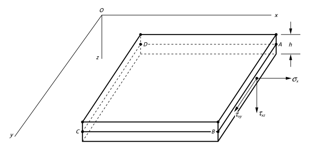
Fig. 2.1 Schematic representation of a plate or shell element of thickness h. Within the context of a shell theory, the actual solid is approximated by its mid-plane (ABCD), and the stresses distributions (\(\sigma_x, \tau_{xy}, \tau_{xz}\)) are replaced by stress resultants along curves in the middle plane (AB for instance in the figure).

In this sense, the shell theory replaces the distributed normal stress \(\sigma_x\) per unit area on the positive x-face of the element by a normal force N_x per unit length along AB, and a bending moment \(M_x\) per unit length along AB that can be expressed as:

(2.5)\[\begin{aligned} N_x = \int_{-h/2}^{h/2} \sigma_x dz \end{aligned}\]

(2.6)\[\begin{aligned} M_x = \int_{-h/2}^{h/2} z \sigma_x dz \end{aligned}\]

These line distributions of force and moment are statically equivalent to the surface distribution \(\sigma_x\). Similarly, the distribution of vertical shear stress \(τ_{xz}\) is statically equivalent to a vertical shear force \(V_x\) per unit length along AB in the form:

(2.7)\[\begin{aligned} V_x = \int_{-h/2}^{h/2} \tau_{xz} dz \end{aligned}\]

And finally, the horizontal shear forces resulting from the shear stress distribution \(\tau_{xz}\) are represented by a twisting moment per unit length of the form:

(2.8)\[\begin{aligned} M_{xy} = - \int_{-h/2}^{h/2} z \tau_{xy} dz \end{aligned}\]

Finally, the horizontal shear forces per unit length \(N_{xy}\) and \(N_{yx}\) are defined as:

(2.9)\[\begin{aligned} N_{xy} = N_{yx} = \int_{-h/2}^{h/2} \tau_{xy} dz \end{aligned}\]

Forces \(N_y\) and \(V_y\) and bending moments \(M_y\) per unit length are defined by replacing \(x\) by \(y\) in the equations above. Fig. 2.2 summarizes the positive sign convention for the stress resultants.

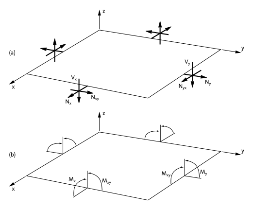
Fig. 2.2 Sign convention for stress resultants. (a) Positive forces. (b) Positive moments.

The forces per unit length (\(N_x\), \(N_y\) and \(N_{xy}\)) acting in the plane of the shell are called membrane forces.

Thus, summarizing, it is possible to define the strengths on the shell as follows:

(2.10)\[\begin{split}\begin{aligned} \hat{\boldsymbol{\sigma}}^{'} = \begin{bmatrix} \hat{\sigma}_m^{'} \\ ... \\ \hat{\sigma}_f^{'} \\ ... \\ \hat{\sigma}_s^{'} \\ \end{bmatrix} = \begin{bmatrix} N_x^{'} \\ N_y^{'} \\ N_{x^{'} y^{'}} \\ ... \\ M_x^{'} \\ M_y^{'} \\ M_{x^{'} y^{'}} \\ ... \\ V_x^{'} \\ V_y^{'} \\ \end{bmatrix} = \int_{-h/2}^{h/2} \begin{bmatrix} \sigma_x^{'} \\ \sigma_y^{'} \\ \tau_{x^{'} y^{'}} \\ ... \\ z^{'} \sigma_x^{'} \\ z^{'} \sigma_y^{'} \\ z^{'} \tau_{x^{'} y^{'}} \\ ... \\ \tau_{x^{'} z^{'}} \\ \tau_{y^{'} z^{'}} \end{bmatrix} dz^{'} = \int_{-h/2}^{h/2} \begin{bmatrix} \boldsymbol{\sigma}_f^{'} \\ ... \\ z^{'} \boldsymbol{\sigma}_f^{'} \\ ... \\ \boldsymbol{\sigma}_s^{'} \end{bmatrix} dz^{'} \end{aligned}\end{split}\]

where \(h\) is the thickness of the shell and \(\hat{\sigma}_m^{'}\), \(\hat{\sigma}_f^{'}\), and \(\hat{\sigma}_s^{'}\) are the membrane, flexural and shear generalized local stresses respectively. The relation between the generalized stresses and the generalized local deformations can be finally obtained from Eqs. (2.2) and (2.10).

(2.11)\[\begin{split}\begin{aligned} \hat{\boldsymbol{\sigma}}^{'} = \begin{bmatrix} \hat{\sigma}_m^{'} \\ ... \\ \hat{\sigma}_f^{'} \\ ... \\ \hat{\sigma}_s^{'} \\ \end{bmatrix} = \int_{-h/2}^{h/2} \begin{bmatrix} \boldsymbol{\sigma}_f^{'} \\ ... \\ z^{'} \boldsymbol{\sigma}_f^{'} \\ ... \\ \boldsymbol{\sigma}_s^{'} \\ \end{bmatrix} dz^{'} = \int_{-h/2}^{h/2} \begin{bmatrix} \boldsymbol{D}_f^{'} \left( \hat{\varepsilon}_m^{'} + z^{'} \hat{\varepsilon}_f^{'} \right) \\ ... \\ z^{'} \boldsymbol{D}_f^{'} \left( \hat{\varepsilon}_m^{'} + z^{'} \hat{\varepsilon}_f^{'} \right) \\ \end{bmatrix} dz^{'} = \hat{\boldsymbol{D}}^{'} \begin{bmatrix} \hat{\varepsilon}_m^{'} \\ ... \\ \hat{\varepsilon}_f^{'} \\ ... \\ \hat{\varepsilon}_s^{'} \\ \end{bmatrix} \end{aligned}\end{split}\]

being \(\hat{\boldsymbol{D}}^{'}\) the shell constitutive matrix.

(2.12)\[\begin{split}\begin{aligned} \hat{\boldsymbol{D}}^{'} = \int_{-h/2}^{h/2} \begin{bmatrix} \boldsymbol{D}_f^{'} & z^{'} \boldsymbol{D}_f^{'} & 0 \\ z^{'} \boldsymbol{D}_f^{'} & {z^{'}}^{2} \boldsymbol{D}_f^{'} & 0 \\ 0 & 0 & \boldsymbol{D}_s^{'} \\ \end{bmatrix} \end{aligned}\end{split}\]

2.1.2.1.1. Stiffened shells model

RamSeries allows to simulate shell structures reinforced with beam elements using a simpler approach consisting on using an equivalent reinforced shell model. The equivalence is achieved by enforcing the equivalent shell to have the same weight, flexural rigidity (i.e. inertia) and membrane stiffness (area) than the original shells/beams structure.

In order to ensure that the equivalent shell has the same weight than the shell-beams system the following relation must be fulfilled:

(2.13)\[\begin{aligned} \rho_{eq} = \rho \cdot h_{eq} \cdot \left( A_{sh} + A_{st} \right) / A_{eq} \end{aligned}\]

where \(sh\) , \(st\) and \(eq\) subscripts refer to the shell, stiffener and equivalent shell quantities respectively.

Following the Reissner-Mindlin formulation in (2.3) and (2.4) and assuming an isotropic material, the flexural and shear stiffness matrices of the equivalent shell can be written as follows:

(2.14)\[\begin{split}\begin{aligned} \boldsymbol{D}_f^{'} = \frac{1}{1 - \nu^2} \begin{bmatrix} E & \nu E & 0 \\ \nu E & E & 0 \\ 0 & 0 & ( 1 - \nu^2 ) G \\ \end{bmatrix} \end{aligned}\end{split}\]

(2.15)\[\begin{split}\begin{aligned} \boldsymbol{D}_s^{'} = \begin{bmatrix} \alpha G & 0 \\ 0 & α G \\ \end{bmatrix} \end{aligned}\end{split}\]

And the stiffness matrix of the system is given by:

(2.16)\[\begin{split}\begin{aligned} \boldsymbol{D}^{'}_{shell} = \begin{bmatrix} D_m & D_{mf} & 0 \\ D_{mf} & D_f & 0 \\ 0 & 0 & D_c \end{bmatrix} \end{aligned}\end{split}\]

where:

(2.17)\[\begin{split}\begin{aligned} \boldsymbol{D}_m = \frac{h \cdot E}{1-\nu^2} \begin{bmatrix} 1 & \nu & 0 \\ \nu & 1 & 0 \\ 0 & 0 & \frac{G (1-\nu^2)}{E} \end{bmatrix} \end{aligned}\end{split}\]

(2.18)\[\begin{split}\begin{aligned} \boldsymbol{D}_f = \frac{E}{12 (1-\nu^2)} \begin{bmatrix} \frac{12 I_{ENshell}}{c} & h^3 \nu & 0 \\ h^3 \nu & h^3 & 0 \\ 0 & 0 & \frac{h^3 G (1-\nu^2)}{E} \end{bmatrix} \end{aligned}\end{split}\]

(2.19)\[\begin{split}\begin{aligned} \boldsymbol{D}_c = h \alpha \begin{bmatrix} G & 0 \\ 0 & G \\ \end{bmatrix} \end{aligned}\end{split}\]

with \(\alpha = 5/6\) and \(\boldsymbol{D}_{mf} = 0\) for simplicity.