1.3.13. Load cases
1.3.13.1. Simple load cases
One load case is a group of one or more loads assigned to entities (point, line, surface or volume). When a new model is defined in RamSeries, a default load case, called Load case 1, is defined. It is possible to rename this load case by double-clicking on the Load case label; it is also possible to define new ones by using the right-click on one of the load cases labels in the tree and choosing the ‘Copy’ option, or right-click on the ‘Loadcases’ label and ‘Create new Loadcase’.
When a load is assigned to one or several entities, this load is inserted inside the load case that is currently active. If combined load cases are not defined, RamSeries calculates just one analysis that is equivalent to that of all the loads belonging to one load case.
1.3.13.2. Combined load cases
Loadcases > Combined LC.
One default combined load case is already existent. To create more, press right mouse button over the existent combined load case name. A menu appears that offers several options. One factor must be entered for every simple load case. This factor will multiply the load in order to create the combined load case. In the post-processing part, after the analysis, there will be one different result for every combined load case. Enter value order to deactivate that load case. The field ELU does not modify the strengths result of the analysis. It is only considered in the concrete section dimension. Its meaning is:
If it is activated, the combined load case is used for calculating the section to collapse. Typically, magnifying factors are bigger than 1.0.
If it is not activated, the combined load case is used for calculating the section in service. Typically, magnifying factors are 1.0.
1.3.13.3. Load case properties
This options are available by double-clicking on each Loadcase name, and indicate whether the load case is a “normal” one, used for applying loads, or if by contrary, will only be used for calculating the center of gravity, weight and other properties of the structure (inertia, total weight and radii of gyration).
1.3.13.4. Waves data
When General data > Marine tools option is activated, it is possible to define wave loads (Morison). Furthermore, it si possible to define a different set of wave characteristics for each Loadcase.
1.3.13.5. Static loads
When a static load is assigned to entities, it is automatically inserted in the active load case. See the load cases section for details.
1.3.13.6. Dynamic loads
When a dynamic load is assigned to an entity (point., line or area), it is automatically added to the active load case inserted in the active load case. See the load cases section for details. Each type of dynamic load has loads have the following options:
Amplitudes: Indicate the amplitude of the dynamic loads.
Parameters: Define the time variation of the dynamic loads variation in time of the dynamic loads.
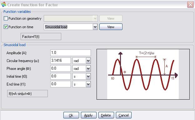
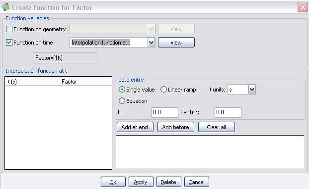
The time variation can be defined using harmonic variations (Sine/Cosine load) or by specifying discrete values in form of a table (Table).
1.3.13.7. Element loads
In the following paragraphs, the different loads that can be applied to the entities are described. Note that some of them are only applicable for some entities.
1.3.13.7.1. Punctual load
This is a load applied to one point of the structure. Default units are Newtons for the force components and Newton·meter for the momentum components. Sign of the components is equal to that defined for the constraints.
1.3.13.7.2. Self weight load
If this condition is applied to a beam, shell element or solid element, the load due to its self-weight is applied, based on the specific weight and other parameters described in the properties. This condition can be applied to either lines for beams, surfaces for shells and volumes for the solid analysis.
1.3.13.7.3. Torque load
It only applies to beams and cables (line entities).
1.3.13.7.4. Pressure load
Beams, cables: A linear pressure (in N/m) is applied to the line.
Shells, solids: A pressure in Pa is applied to the surface (surface face for solids).
There are three types of pressure loads for beams:
Global beam load.
Global projected beam load.
Local beam load.
In all the cases the pressure applied is given in Newton/meter in default units. In the global load, the load is given related to the global axes. The global projected load is given also in global axes but the length considered of the beam is orthogonal to the load. Local load is related to the local axes defined in the properties section.
In the Local beam load there is an additional field that is the local torque momentum.
1.3.13.7.5. Shell pressure load
There are five types of surface loads for shells:
Global shell load.
Global projected shell load.
Local shell load.
Triangular load.
Hydrostatic load.
In all the cases the pressure applied is given in Newton/meter2 in default units. In the global load, the load is given related to the global axes. The global projected load is given also in global axes but the area considered of the shell is orthogonal to the load. Local load is related to the local axes defined in the properties section.
Triangular load is like a Global shell load but with a triangular variation in its values. It is defined by two points, given by its coordinates, and pressure values associated to each one of these points. The pressure assigned to the elements that project between the points is a linear interpolation between the two values. The elements that project outside have a pressure value of zero.
Example:
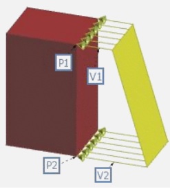
Fig. 1.38 Diagram of how triangle loads are defined.
Hydrostatic load is defined related to the gravity direction entered in the problem data section. The reference coordinate is related to that direction. Self-weight water is given, in default units as N/m3. Note that the direction of the acting pressure will be the normal to the surface on which it is applied, but the the sense will be the opposite to that of this normal to the surface.
1.3.13.7.6. Shell boundary pressure load
With this condition it is possible to apply a pressure to a line that is a boundary of a shell surface. The pressure is given in default units in N/m. If the local axes field is set to Global, the pressure vector is given related to the global axes. Option Automatic permits to define an automatic local axes system that is different for every element. Pressure vector will be related to these axes. This last option is useful to assign a local pressure to the boundary of the shell.
Check: Data > Local axes > Surfaces > Draw
to see the automatic local axes defined. Triangular and hydrostatic face load are defined equal to the ones in shell surface loads.
1.3.13.7.7. Solid surface load
There are five types of surface loads for solids:
Global pressure load.
Global projected pressure load.
Local pressure load.
Triangular load.
Hydrostatic load.
In all the cases the pressure applied is given in Newton/meter2 in default units. In the global load, the load is given related to the global axes. The global projected load is given also in global axes but the area considered of the contour of the solid is orthogonal to the load. Local load has only one component and it is the normal pressure to the contour surface. Its value is positive when the pressure points inwards the volume.
Triangular and hydrostatic loads are defined equal to the ones in shell surface loads.
1.3.13.7.8. Thermal strain load
It is possible to define for every beam, shell or solid, a load due to changes in temperature. The values to enter are:
Alpha (α): The constant expressed in \(^\circ C^{-1}\) (Celsius degrees).
Delta T (ΔT): Temperature increment in Celsius degrees.
The deformation (\(\varepsilon\))added to the beam, shell or solid, is:
1.3.13.7.9. Strain load
It is possible to define for every beam, shell or solid, a load due to linear changes in certain magnitude. The values to enter are:
Alpha (α): The constant expressed in 1/ΔU.
Delta U (ΔU): Magnitude increment.
The deformation (\(\varepsilon\)) added to the beam, shell or solid is:
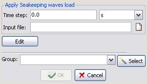
1.3.13.7.10. SeaFEM waves load
Allows to use as a pressure load the result of a previously calculated SeaFEM analysis (Input file), at a certain Time step. This load applies over shell elements.
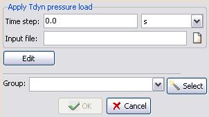
1.3.13.7.11. Tdyn pressure load
Allows to use as a pressure load the result of a previously calculated Tdyn analysis (Input file), at a certain Time step. This load applies over shell elements.
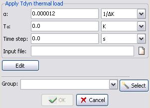
1.3.13.7.12. Tdyn thermal load
Allows to use the result of a previously calculated Tdyn heat transfer analysis (Input file), at a certain Time step, to create a thermo-mechanical strain. This load applies over solid elements.
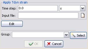
1.3.13.7.13. Tdyn strain load
Allows to use the result of a previously calculated Tdyn URSOLVER analysis (Input file), at a certain Time step, to create a mechanical strain. This load applies over solid elements.