2.3.9. Mooring

2.3.9.1. Mooring system modelling

SeaFEM can handle complex mooring systems made up of various mooring lines attached to the floating structure. Each mooring line can be in turn composed of various segments each one resembling a chain, a steel cable or even a synthetic fiber. Forces resulting from the action of buoys and sinkers acting at the junctions between mooring line segments can also be considered. Hence, SeaFEM can deal with a wide variety of multi-segmented mooring line systems. Cable tensions depend on the buoyancy and lateral displacements of the floating structure, the cable weight in water, the elasticity in the cable and the geometrical layout of the mooring system. Hence, as the floating structure moves in response to unsteady environmental loadings, the mooring restraining forces change with the changing cable tension. This means that the mooring system has an effective compliance whose response is in general non-linear. Within SeaFEM, mooring inertia and damping are ignored, but the non-linear response is accounted for in the mooring system dynamics. Mooring systems within SeaFEM are solved using a quasi-static approach in the sense that at any step of the calculation, and once the floating body displacements are known, the mooring system solver calculates the tensions and the geometrical configuration of each mooring line segment assuming that each cable is in static equilibrium at that instant. The mooring loads resulting from the calculation are added to the total load acting on the floating body, and the resulting dynamic equations of motion of the structure are solved again until convergence. At each time step the implicit non-linear system of equations describing the mooring system is solved using a classical Newton-Raphson scheme. The formulation implemented within SeaFEM for dealing with catenary based mooring systems is outlined in what follows. Additionally, cables behaving as springs (both in tension and/or compression) can also be modeled.

2.3.9.1.1. Catenary equations

In a local coordinate system with its origin located at the lower cable point, the mooring equations for the catenary read as follows:

(2.620)\[\begin{aligned} & z = \left( \frac{T_o}{\Omega} \right) cosh \left( \frac{\Omega}{T_o} x + α \right) + β \end{aligned}\]

(2.621)\[\begin{aligned} & s = \left( \frac{T_o}{\Omega} \right) sinh \left( \frac{\Omega}{T_o} x + α \right) + \Gamma \end{aligned}\]

where \(z\) is the vertical position, \(s\) is the catenary arc length, \(\Omega\) is the catenary weight per unit length in water, and \(T_o\) is the horizontal component of the cable tension which is constant everywhere. If the conditions \(z(x=0)=0\) and \(s(x=0)=0\) are applied, the equations result to be:

(2.622)\[\begin{aligned} & z = \left( \frac{T_o}{\Omega} \right) \left[ cosh \left( \frac{\Omega}{T_o} x + α \right) - cosh \left( \alpha \right) \right] \end{aligned}\]

(2.623)\[\begin{aligned} & s = \left( \frac{T_o}{\Omega} \right) \left[ sinh \left( \frac{\Omega}{T_o} x + α \right) - sinh \left( \alpha \right) \right] \end{aligned}\]

The action of any part of the line upon its neighbor is purely tangential, and the tangential direction can be written as:

(2.624)\[\begin{aligned} & tan \theta = \frac{dz}{dx} = sinh \left( \frac{\omega}{T_o} x + \alpha \right) \end{aligned}\]

The equilibrium equations can be written as:

(2.625)\[\begin{aligned} & T_{down} \cdot cos\theta_{down} = T_{up} \cdot cos\theta_{up} = T_o \end{aligned}\]

(2.626)\[\begin{aligned} & T_{up} \cdot sin\theta_{up} - T_{down} \cdot sin\theta_{down} = \Omega\cdot L \end{aligned}\]

From the horizontal component of the tension at any point of the catenary, it is possible to write the modulus of the cable tension at any point of the catenary as:

(2.627)\[\begin{aligned} & T = \frac{T_o}{cos\theta} = T_o \cdot \left( \sqrt{1+tan^2 \theta} \right) = T_o \cdot cosh \left( \frac{\Omega}{T_o} x + α \right) \end{aligned}\]

Hence, the vertical component of tension at any point of the catenary can be written as:

(2.628)\[\begin{aligned} & T_v = T \cdot sin\theta = T_o \cdot sinh \left( \frac{\Omega}{T_o} x + α \right) \end{aligned}\]

In particular, at the upper and bottom vertex of the catenary above equation reads, respectively:

(2.629)\[\begin{aligned} & T_{v up} = T_o \cdot sinh \left( \frac{\Omega}{T_o} l + α \right) \end{aligned}\]

(2.630)\[\begin{aligned} & T_{v down} = T_o \cdot sinh \left(α \right) \end{aligned}\]

and the vertical equilibrium equation will result in:

(2.631)\[\begin{aligned} & L = \left( \frac{T_o}{\Omega} \right) \left( sinh \left( \frac{\Omega}{T_o} l + α \right) - sinh⁡(α) \right) = s(x=l) \end{aligned}\]

For a given length of the catenary \((L)\) and for given horizontal and vertical distances \((l,h)\) between the initial and end points of the catenary, it is possible to solve the equations by using a classical Newton-Raphson iterative process. If the catenary has a seabed contact in its lower point, the following condition must be added

(2.632)\[\begin{aligned} & \frac{dz}{dz} |_{x=0} = 0 \end{aligned}\]

and the catenary equations result in:

(2.633)\[\begin{aligned} & z = \left( \frac{T_o}{\Omega} \right) \left[ cosh \left(\frac{\Omega}{T_o} x \right)-1 \right] \end{aligned}\]

(2.634)\[\begin{aligned} & s = \left( \frac{T_o}{\Omega} \right) \left[ sinh \left(\frac{\Omega}{T_o} x \right)\right] \end{aligned}\]

2.3.9.1.2. Dynamic cable formulation

SeaFEM includes a finite element model (FEM) for solving mooring line dynamics. For this purpose, the line is divided into a series of straight segments modeled by nonlinear truss elements, with three translational degrees of freedom per node. Lagrangian formulation is used to describe the dynamics of the mooring line.

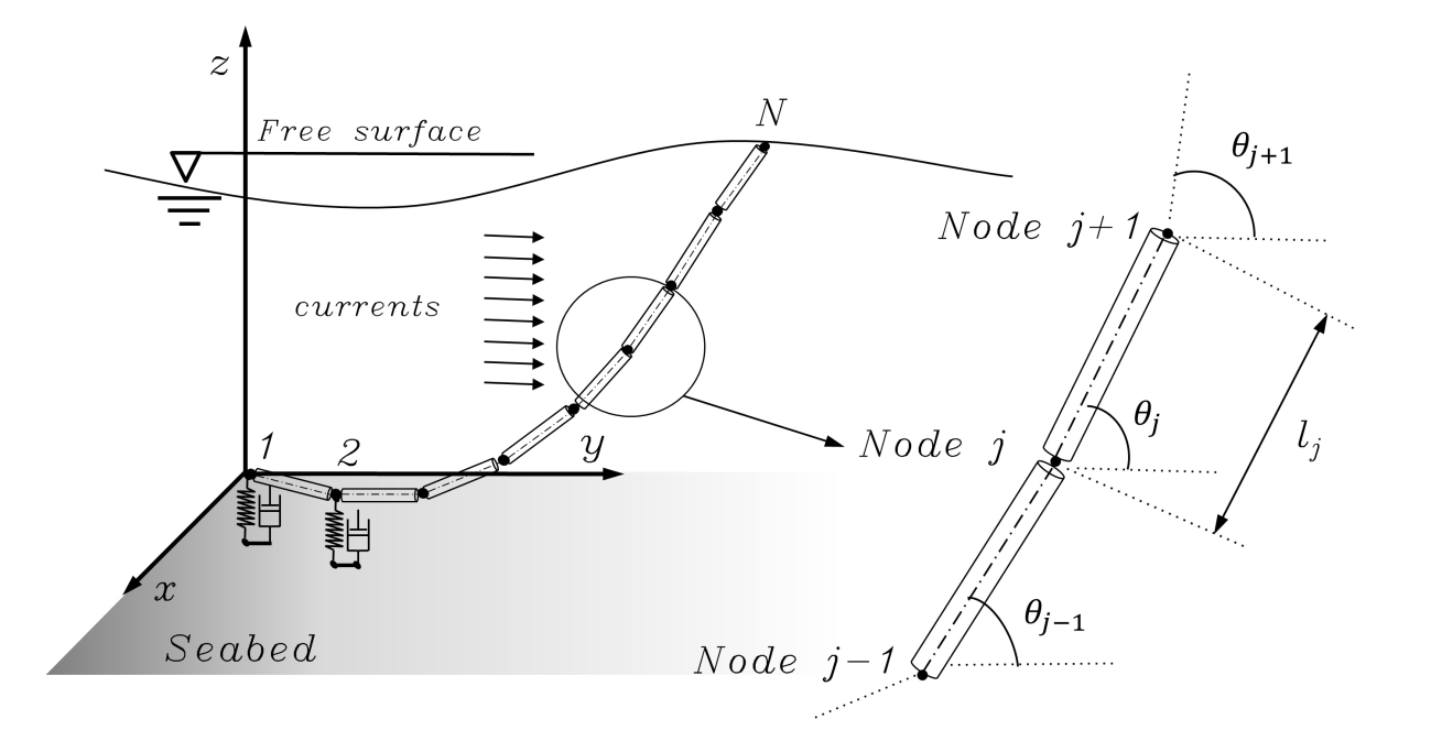
Fig. 2.23 Scheme of the FEM cable model

Applying FEM formulation to this nonlinear elastodynamics problem, the equations of the dynamics of the line can be written as follows:

(2.635)\[\begin{aligned} & \left( \overline{\overline{\boldsymbol{M}}}^{t+dt} + \overline{\overline{\boldsymbol{M}}}_A^{t+dt} \right) \ddot{x} + \overline{\overline{C}}^{t+dt} \dot{x}+ \boldsymbol{P}^0 + \boldsymbol{R}^{t+dt} = \boldsymbol{F}^{t+dt} \end{aligned}\]

where \(x\) is the vector of nodal translational degrees of freedom, \(\boldsymbol{F}\) the vector of external loads, \(\overline{\overline{\boldsymbol{M}}}`the inertia matrix of the line, :math:\)overline{overline{boldsymbol{M}_A}}` the added mass matrix, \(\boldsymbol{P}^0\) is the pretension vector in the initial configuration, and \(\boldsymbol{R}\), the vector of internal forces of the cable. Damping effects of mooring cable can be inserted through a Rayleigh-type damping matrix \(\overline{\overline{\boldsymbol{C}}}\). Considering the standard linearization of the internal forces, above equations can be expressed as:

(2.636)\[\begin{aligned} & \left( \overline{\overline{\boldsymbol{M}}}^{t+dt} + \overline{\overline{\boldsymbol{M}_A}}^{t+dt} \right) \ddot{\boldsymbol{x}} + \overline{\overline{\boldsymbol{C}}}^{t+dt} \dot{\boldsymbol{x}} + \boldsymbol{P}^0 + \left( \overline{\overline{\boldsymbol{K}}}^{t+dt} + \overline{\overline{\boldsymbol{K}_G}}^{t+dt} \right) \Delta x + \boldsymbol{R}^t = \boldsymbol{F}^{t+dt} \end{aligned}\]

where \(\overline{\overline{\boldsymbol{K}}}\) and \(\overline{\overline{\boldsymbol{K}_G}}\) are the so called material stiffness matrix and geometric stiffness matrix, respectively [7]. The corresponding elemental material stiffness matrix \(\overline{\overline{\boldsymbol{k}}}^e\), and geometric stiffness matrix, \(\overline{\overline{\boldsymbol{k}_G}}^e\), can be obtained in terms of the strain of the truss element, \(e\):

(2.637)\[\begin{aligned} & \overline{\overline{\boldsymbol{k}^e}} + \overline{\overline{\boldsymbol{k}_G^e}} = \frac{\partial }{\partial x} \left( V^e s \frac{\partial e}{\partial x} \right) = V^e E \frac{\partial e}{\partial x} ⊗ \frac{\partial e}{\partial x} + V^e s \frac{\partial ^2 e}{\partial x^2} \end{aligned}\]

where \(V^e\) is the volume of the element, \(s\) the axial stress and \(E\) the axial elastic modulus. The FEM allows calculating those matrixes as follows [8]

(2.638)\[\begin{split}\begin{aligned} & \overline{\overline{\boldsymbol{k}^e}} = V^e E \frac{\partial e}{\partial x} ⊗ \frac{\partial e}{\partial x} = \int_0^{le} B_o^T V^e EB_o ds \\ & \overline{\overline{\boldsymbol{k}_G^e}} = V^e f \frac{\partial^2 e}{\partial x^2} = \int_0^{le} B_l^T SB_l ds \end{aligned}\end{split}\]

The elemental inertia matrixes are evaluated as:

(2.639)\[\begin{aligned} & \overline{\overline{\boldsymbol{m}^e}} = \int_0^{le} \overline{\overline{\boldsymbol{N}^T}} \rho \overline{\overline{\boldsymbol{N}}} ds \end{aligned}\]

and the added mass matrix is calculated as

(2.640)\[\begin{aligned} & m_a^e = \rho A C_m \int_0^{le} \overline{\overline{\boldsymbol{N}^T}} \overline{\overline{\boldsymbol{N}}} ds \end{aligned}\]

In the above equations, \(\overline{\overline{\boldsymbol{N}}}\) is the general matrix of shape functions [8], \(A\) is the section area of the cable, and \(C_m\) is the added mass coefficient. Finally, the damping matrix is evaluated using the Rayleigh formulation:

(2.641)\[\begin{aligned} & \overline{\overline{\boldsymbol{C}}} = a_1 \overline{\overline{\boldsymbol{K}}} + a_2 \overline{\overline{\boldsymbol{M}}} \end{aligned}\]

The coefficients \(a_1\), \(a_2\) can be calculated as:

(2.642)\[\begin{aligned} & ζ_i = \frac{1}{2} \left( \frac{a_1}{\Omega_i} + a_2 \Omega_i \right) \end{aligned}\]

where \(ζ_i\) is the damping ratio corresponding to the natural frequency \(\Omega_i\) of the structure. The external forces vector is evaluated by assembling the contribution of the different forces acting on the element:

(2.643)\[\begin{aligned} & \boldsymbol{F}^e = \boldsymbol{F}_w^e + \boldsymbol{F}_h^e + \boldsymbol{F}_d^e + \boldsymbol{F}_f^e + \boldsymbol{F}_o^e \end{aligned}\]

where \(\boldsymbol{F}_w^e\) is the weight, \(\boldsymbol{F}_h^e\) is the buoyancy force, \(\boldsymbol{F}_d^e\) is the drag force related to the currents, \(\boldsymbol{F}_f^e\) is the force due to the seabed interaction and \(\boldsymbol{F}_o^e\) is the drag force due to the waves. The weight and buoyancy force are calculated as follows

(2.644)\[\begin{split}\begin{aligned} & \boldsymbol{F}_w^e + \boldsymbol{F}_h^e = \int_0^{le} f_{wh}^e \overline{\overline{\boldsymbol{N}}} ds \\ & f_{wh}^e = f_w + f_h = g \frac{w(\rho _c - \rho _a)}{(1+e)\rho _c} \end{aligned}\end{split}\]

where \(\rho _c\) is the density of the cable, \(\rho _a\) is the water density, \(w\) weight per meter and \(e\) the strain of the considered element. On the other hand, the drag force acting on the element, is evaluated as

(2.645)\[\begin{split}\begin{aligned} & \boldsymbol{F}_d^e + \boldsymbol{F}_o^e = \int_0^{le} f_{d}^e \overline{\overline{\boldsymbol{N}}} ds \\ & f_d^e = \int_0^{le} \frac{1}{2} \rho C_{Dt} D|U_r^e|U_r^e ds + \int_0^{le} \frac{1}{2} \rho C_{Dn} D|U_r^e|U_r^e \end{aligned}\end{split}\]

where \(D\) is the characteristic diameter of the element, \(C_{Dt}\) and \(C_{Dn}\) the tangential and normal drag coefficients and \(U_r^e\) is the velocity relative to the element. The seabed interaction is modeled with the spring and normal and tangential damping terms given by:

(2.646)\[\begin{aligned} & F_f^e = \int_0^{le} f_{ms}^e \overline{\overline{N}} ds + \int_0^{le}f_{dn}^e \overline{\overline{N}} ds + \int_0^{le} f_{dt}^e \overline{\overline{N}} ds \end{aligned}\]

where the vertical forces per unit length, due to the stiffness of the seabed \(f_{ms}^e\), are expressed as

(2.647)\[\begin{split}\begin{aligned} & f_{ms}^e = \left\{ \begin{matrix} f_1 wl & \text{, if } K_f \left[ z_r - (z^e)^{t+dt} \right] < f_1 wl \\ K_f \left[ z_r - (z^e)^{t+dt} \right] & \text{, if } K_f \left[ z_r - (z^e)^{t+dt} \right] > f_1 wl \\ \end{matrix} \right\} \end{aligned}\end{split}\]

where \(z^e\) is the vertical coordinate of the corresponding node, \(l\) is the length of the cable associated to the node, and \(f_l\) is a coefficient of the model. \(K_f\) is the coefficient of the seabed normal stiffness force which has the magnitude:

(2.648)\[\begin{aligned} & K_f = G_k Dl \end{aligned}\]

where \(D\) is the diameter of the line, and \(G_k\) is the ground normal stiffness per unit length. The term \(z_r\) is then evaluated as:

(2.649)\[\begin{aligned} & z_r = z_i + \frac{wl}{G_k D} \end{aligned}\]

The seabed damping forces are applied in the normal and tangential directions. The normal damping force is only applied when the penetrating object is travelling into the seabed. It is applied in the seabed outwards direction and has a magnitude given by:

(2.650)\[\begin{split}\begin{aligned} & f_{dn}^e = \left\{ \begin{matrix} D_n \dot{z}^e & \text{, if } \dot{z}^e < 0 \\ 0 & \text{, if } \dot{z}^e > 0 \\ \end{matrix} \right\} \end{aligned}\end{split}\]

where \(D_n\) is formulated as a fraction, \(G_c\), of the critical damping as follows:

(2.651)\[\begin{aligned} & D_n=2.0 G_c \sqrt{ G_k \left( \frac{wl^e}{g} \right) Dl^e } \end{aligned}\]

Finally, the tangential damping force is again evaluated as a fraction, \(G_u\), of the critical damping, and is applied in the direction opposing the tangential component of the velocity of the penetrator:

(2.652)\[\begin{split}\begin{aligned} & f_{dt}^e = D_t \dot{x}^e \\ & D_t = 2.0 G_c \sqrt{ G_k \left( \frac{wl^e}{g} \right) Dl^e } \end{aligned}\end{split}\]

An implicit time integration scheme based on called Bossak-Newmark method [2] is applied to solve the system. It will lead to a system of algebraic equations to be solved in iterative manner:

(2.653)\[\begin{split}\begin{aligned} & \left[ (1-α) \left(\overline{\overline{\boldsymbol{M}}}^{t+dt,i} + \overline{\overline{M}}_A^{t+dt,i} \right) + dt \Gamma \overline{\overline{C}}^{t+dt,i} + dt^2 β \left( \overline{\overline{\boldsymbol{K}}}^{t+dt,i} + \overline{\overline{\boldsymbol{K}}}_G^{t+dt,i} \right) \right] \ddot{\boldsymbol{x}}^{t+dt,i+1} = \\ & = dt^2 β \left( \overline{\overline{\boldsymbol{K}}}^{t+dt,i} + \overline{\overline{\boldsymbol{K}}}_G^{t+dt,i} \right) \ddot{\boldsymbol{x}}^{t+dt,i} + \boldsymbol{F}^{t+dt,i} - \boldsymbol{P}^0 + \boldsymbol{R}^t - \\ & - \overline{\overline{C}}^{t+dt,i} \left[ \dot{\boldsymbol{x}}^t - dt (\Gamma +1) \ddot{\boldsymbol{x}}^t \right] - α \left( \overline{\overline{\boldsymbol{M}}}^{t+dt,i} + \overline{\overline{\boldsymbol{M}}}_A^{t+dt,i} \right) \ddot{\boldsymbol{x}}^t \end{aligned}\end{split}\]

where \(dt\) is time step, \(i\) denotes iteration, \(α\) is a parameter related with Bossak-Newmark implicit method, and \(\Gamma ` and :math:`β\) are parameters related to Newmark time integration scheme. Finally, the new position and velocity of each node can be evaluated as:

(2.654)\[\begin{split}\begin{aligned} & x^{t+\Delta t} = x^t + dt \dot{x}^t + \frac{dt^2}{2} \left[(1-2β) \ddot{x}^t + 2β \ddot{x}^{t+dt} \right] \\ & \dot{x}^{t+\Delta t} = \dot{x}^t + dt \left[(1-\Gamma ) \ddot{x}^t + \Gamma \ddot{x}^{t+dt} \right] \end{aligned}\end{split}\]

The dynamic cable solver is integrated within SeaFEM dynamic solver. The scheme of the dynamics solver is presented in the section 7. In order to accelerate the scheme, the mooring forces are linearized within the body dynamics group, by evaluating the stiffness matrix \(K_M\) of the line. A detailed description of the FEM cable model implemented in SeaFEM can be found in [9].