2.3.5. Numerical models (Part II)

2.3.5.1. Stream line integration

The first order free surface boundary conditions can be written in a general, regardless whether the convective velocity has been linearized or not, as follows

(2.536)\[\begin{aligned} & \frac{\partial \phi}{\partial t} + \boldsymbol{U} \cdot \nabla_h \phi + \frac{P_{fs}}{\rho } + g η + R = 0 \end{aligned}\]

(2.537)\[\begin{aligned} & \frac{\partial η}{\partial t} + \boldsymbol{U} \cdot \nabla_h η - \frac{\partial \phi}{\partial z} + S = 0 & \text{in } z = 0 \end{aligned}\]

Where \(R\) and \(S\) represent some remaining terms. The numerical schemes adopted for solving the kinematic-dynamic free surface boundary conditions are based on Adams-Bashforth-Moulton schemes, using an explicit scheme for the kinematic condition, and implicit one for the dynamic condition. Then \(\phi^{n+1}\) is imposed as a Dirichlet boundary condition. The schemes read as follows:

(2.538)\[\begin{aligned} & \phi^{n+1} + \Delta t \left( \boldsymbol{U} \cdot \nabla_h \phi \right)^{n+1} = \phi^n - \Delta t \left(\frac{1}{\rho } P_{fs}^{n+1} - g η^{n+1} - R^{n+1} \right) & \text{in } z = 0 \end{aligned}\]

(2.539)\[\begin{aligned} & η^{n+1} = η^n - \Delta t \left( \boldsymbol{U} \cdot \nabla_h η \right)^n + \Delta t \left(\phi_z^n - S^n \right) & \text{in } z = 0 \end{aligned}\]

where \(\boldsymbol{U}\) is the convective velocity. The convective term is obtained by differentiating along streamlines:

(2.540)\[\begin{aligned} & \left( \boldsymbol{U} \cdot \nabla_h \phi \right)^{n+1} = |\boldsymbol{U}|^{n+1} \partial _L \phi^{n+1} \end{aligned}\]

(2.541)\[\begin{aligned} & \left( \boldsymbol{U} \cdot \nabla_h η \right)^n = |\boldsymbol{U}|^n \partial _L η^n \end{aligned}\]

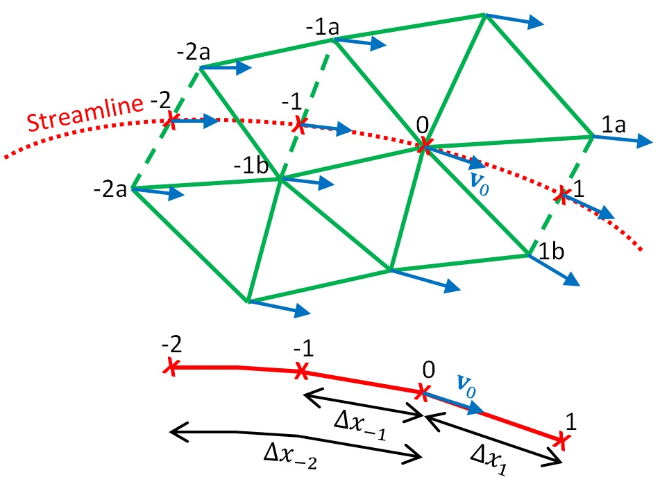
where \(\partial _L\) denotes the derivative along the streamline. This streamline derivative is estimated using a two points upstream and one point downstream differential operator. Figure 5 shows the tracing of the streamline at node \(C\). The left \((-1)\) and forward left \((-2)\) points are the upstream points, while the right \((1)\) point corresponds to the downstream point. The values of the scattered velocity potential \(\phi\) and scattered free surface elevation \(η\) at \(-1\), \(-2\) and \(1\) points are obtained by linear interpolation between the nodes of the edges where they lie on. The stream line differential operator reads as:

(2.542)\[\begin{aligned} & \partial _L \phi_0 = w_1 \phi_1 + w_0 \phi_0 + w_{-1} \phi_{-1} + w_{-2} \phi_{-2} \end{aligned}\]

(2.543)\[\begin{aligned} & \partial _L η_0 = w_1 η_1 + w_0 η_0 + w_{-1} η_{-1} + w_{-2} η_{-2} \end{aligned}\]

where \(\phi _1\), \(\phi _{-1}\), \(\phi _{-2}\) are interpolated between \((\phi{_1a},\phi{_1b} )\), \((\phi_{-1a},\phi_{-1b} )\), and \((\phi_{-2a},\phi_{-2b} )\) respectively. In matrix form:

(2.544)\[\begin{aligned} & \left( \overline{\overline{\boldsymbol{I}}} + \Delta t \overline{\overline{\boldsymbol{W}}}^{n+1} \right) \phi^{n+1} = \overline{\overline{\boldsymbol{I}}} \left( \phi^n - \Delta t \left( \frac{1}{\rho } P_{fs}^{n+1} - g η^{n+1} - R^{n+1} \right) \right) & \text{in } z = 0 \end{aligned}\]

(2.545)\[\begin{aligned} & \overline{\overline{\boldsymbol{I}}} η^{n+1} = \left( \overline{\overline{\boldsymbol{I}}} - \Delta t \overline{\overline{\boldsymbol{W}}}^n \right) η^n + \Delta t \left( \phi_z^n - S^n \right) & \text{in } z = 0 \end{aligned}\]

Where \(\overline{\overline{\boldsymbol{W}}}\) is the streamline convective matrix, and \(\overline{\overline{\boldsymbol{I}}}\) is the identity matrix. The stencils are obtained using Taylor series expansion to impose a second order finite difference scheme along the streamline. That is to say, solving the following system of equations:

(2.546)\[\begin{aligned} & w_1 + w_0 + w_{-1} + w_{-2} = 0 \end{aligned}\]

(2.547)\[\begin{aligned} & w_1 \Delta x_1 - w_{-1} \Delta x_{-1} - w_{-2} \Delta x_{-2} = 1 \end{aligned}\]

(2.548)\[\begin{aligned} & w_1 \frac{\Delta x_1^2}{2} + w_{-1} \frac{\Delta x_{-1}^2}{2} + w_{-2} \frac{\Delta x_{-2}^2}{2} = 0 \end{aligned}\]

(2.549)\[\begin{aligned} & w_1 \frac{\Delta x_1^3}{6} - w_{-1} \frac{\Delta x_{-1}^3}{6} -w_{-2} \frac{\Delta x_{-2}^3}{6} = 0 \end{aligned}\]

Fig. 2.20 Streamline discretization

The associated matrix form to the finite element formulation for the governing equations is:

(2.550)\[\begin{aligned} & \overline{\overline{\boldsymbol{L}^*}} \phi = \boldsymbol{b}^(Z_0 ) + \boldsymbol{b}^B + \boldsymbol{b}^R \end{aligned}\]

where \(\overline{\overline{\boldsymbol{L}^*}}\) is the standard laplacian matrix modified to account for the left hand side of Eq.(5 7), \(\boldsymbol{b}^(Z_0 )\) is a vector accounting for the right hand side of Eq. (5 7), and \(\boldsymbol{b}^B\) and \(\boldsymbol{b}^R\) are the vectors resulting of integrating the corresponding boundary condition terms.

2.3.5.2. Streamline Upwind Petrov-Galerkin (SUPG) formulation

Alternatively, a SUPG stabilization scheme is also available in SeaFEM for the integration of the free surface boundary conditions. Both, the dynamic and kinematic boundary conditions can be seen as a convection-reaction equation:

(2.551)\[\begin{aligned} & \frac{\partial χ}{\partial t} + \boldsymbol{U} \cdot \nabla_h χ + Q = 0 \end{aligned}\]

Weak formulation:

(2.552)\[\begin{aligned} & \int_\Omega W \left( \frac{\partial χ}{\partial t} + \boldsymbol{U} \cdot \nabla_h χ + Q \right) dσ = 0 \end{aligned}\]

Discrete Galerkin method:

(2.553)\[\begin{aligned} & ∀i \int_\Omega N^i \left( N^j \frac{\partial χ_j}{\partial t} + \boldsymbol{U} \cdot \nabla_h N^j χ_j + N^j Q_j^{n+\theta} \right) dσ = 0 \end{aligned}\]

Time marching scheme:

(2.554)\[\begin{split}\begin{aligned} & ∀i \int_\Omega N^i N^j \frac{χ_j^{n+1} - χ_j^n}{\Delta t} dσ + \int_\Omega N^i \left( \boldsymbol{U}^{n+1}\cdot \nabla_h N^j \right) χ_j^{n+\theta} dσ + \\ & + \int_\Omega N^i N^j Q_j^{n+\theta} dσ = 0 \end{aligned}\end{split}\]

SUPG Stabilization:

(2.555)\[\begin{split}\begin{aligned} & ∀i \sum_e \left\{ \begin{matrix} \int_{\Omega^e} N^i N^j \frac{χ_j^{n+1} - χ_j^n}{\Delta t} dσ + \int_{\Omega^e} N^i \left( \left( \boldsymbol{U}^e \right)^{n+\theta} \cdot \nabla_h N^j \right) χ_j^{n+\theta} dσ \\ + \int_{\Omega^e} N^i N^j \left( \frac{P_j^{n+\theta}}{\rho } + gη_j^{n+\theta} + R_j^{n+\theta} \right) dσ \\ \end{matrix} \right\} + \\ & \sum_e \frac{h_e (U^e)^{n+\theta}}{2|(U^e)^{n+\theta}|} \left\{ \begin{matrix} [\int_{\Omega^e}\nabla_h N^i N^j dσ] \frac{χ_j^{n+1}-χ_j^n}{\Delta t} + [\int_{\Omega^e}\nabla_h N^i ((\boldsymbol{U}^e )^(n+α)\cdot\nabla_h N^j )dσ] χ_j^{n+\theta}\\ + [\int_{\Omega^e}\nabla_h N^i N^j dσ] Q_j^{n+\theta} \\ \end{matrix} \right\} = 0 \end{aligned}\end{split}\]

where \(({U^e})^{n+\theta}\) is the average convective velocity within the element, and \((U^e )^{n+α} = \sum_{k_e}N^{k_e } U_{k_e}^{n+α}\) . Reordering terms:

(2.556)\[\begin{split}\begin{aligned} & ∀i \sum_{e,i_e,j_e}\Big[\int_{\Omega^e}N^{i_e } N^{j_e } dσ + \frac{h_e (U^e)^{n+\theta}}{2} |(U^e)^{n+\theta}| \\ & \int_{\Omega^e}\nabla_h N^{i_e } N^{j_e } dσ \Big] χ_j^{n+1} -\sum_{e,i_e,j_e} \Big[\int_{\Omega^e}N^{i_e } N^{j_e } dσ \\ & + (h_e (U^e)^{n+\theta})/2|(U^e)^{n+\theta} | \int_{\Omega^e}\nabla_h N^{i_e } N^{j_e } dσ \Big] χ_j^n = \\ & -\Delta t \sum_(e,i_e,j_e) \Big[\int_{\Omega^e}N^i (N^{k_e } U_{k_e}^{n+\theta}\cdot\nabla_h N^{j_e } ) dσ \\ & + (h_e (U^e)^{n+\theta})/2|(U^e)^{n+\theta}| \int_{\Omega^e}\nabla_h N^{i_e } (N^{k_e } U_{k_e}^{n+\theta}\cdot\nabla_h N^{j_e } ) dσ \Big] χ_j^{n+\theta} \\ & -\Delta t\sum_{e,i_e,j_e} \Big[\int_{\Omega^e}N^{i_e } N^{j_e } dσ+(h_e (U^e)^{n+\theta})/2|(U^e)^{n+\theta}| \int_{\Omega^e}\nabla_h N^{i_e } N^{j_e } dσ \Big] Q_j^{n+\theta} \end{aligned}\end{split}\]

In matrix form:

(2.557)\[\begin{split}\begin{aligned} & (\overline{\overline{\boldsymbol{M}}}+\overline{\overline{\boldsymbol{M}}}_{supg}^{n+\theta} ) χ^{n+1}+\Delta t(\overline{\overline{\boldsymbol{C}}}^{n+\theta}+\overline{\overline{\boldsymbol{C}}}_{supg}^{n+\theta} ) \thetaχ^{n+1} = \\ & (\overline{\overline{\boldsymbol{M}}}+\overline{\overline{\boldsymbol{M}}}_{supg}^{n+1} ) χ^n-\Delta t(\overline{\overline{\boldsymbol{C}}}^{n+\theta}+\overline{\overline{\boldsymbol{C}}}_{supg}^{n+\theta} ) (1-\theta)χ^n+(\overline{\overline{\boldsymbol{M}}}+\overline{\overline{\boldsymbol{M}}}_{supg}^{n+1} ) Q^{n+\theta} \end{aligned}\end{split}\]

where:

(2.558)\[\begin{aligned} & \overline{\overline{\boldsymbol{M}}} = \sum_{e,i_e,j_e}\int_{\Omega^e}N^{i_e } N^{j_e } dσ \end{aligned}\]

(2.559)\[\begin{aligned} & \overline{\overline{\boldsymbol{M}}}_{supg}^{n+\theta}=\sum_{e,i_e,j_e}[\frac{h_e (\boldsymbol{U}^e)^{n+\theta}}{2} |(\boldsymbol{U}^e)^{n+\theta} | \int_{\Omega^e}\nabla_h N^{i_e } N^{j_e } dσ] \end{aligned}\]

(2.560)\[\begin{aligned} & \overline{\overline{\boldsymbol{C}}}^{n+\theta}=\sum_{e,i_e,j_e}\int_{\Omega^e}N^i (N^{k_e } \boldsymbol{U}_{k_e}^{n+\theta} \cdot \nabla_h N^{j_e } ) \end{aligned}\]

(2.561)\[\begin{aligned} & \overline{\overline{\boldsymbol{C}}}_{supg}^{n+\theta}=\sum_{e,i_e,j_e}[\frac{h_e (U^e)^{n+\theta}}{2}|(U^e)^{n+\theta} | \int_{\Omega^e}\nabla_h N^{i_e } (N^{k_e } U_{k_e}^{n+\theta}\cdot\nabla_h N^{j_e } ) dσ] \end{aligned}\]

Following the same procedure as for the convection-reaction equation, the dynamic boundary condition becomes:

(2.562)\[\begin{split}\begin{aligned} & (\overline{\overline{\boldsymbol{M}}}+\overline{\overline{\boldsymbol{M}}}_{supg}^{n+\theta} ) ϕ^{n+1}+\Delta t(\overline{\overline{\boldsymbol{C}}}^{n+\theta}+\overline{\overline{\boldsymbol{C}}}_{supg}^{n+\theta} ) \thetaϕ^{n+1} = \\ & (\overline{\overline{\boldsymbol{M}}}+\overline{\overline{\boldsymbol{M}}}_{supg}^{n+1} ) ϕ^n-\Delta t(\overline{\overline{\boldsymbol{C}}}^{n+\theta}+\overline{\overline{\boldsymbol{C}}}_{supg}^{n+\theta} ) (1-\theta)ϕ^n-(\overline{\overline{\boldsymbol{M}}}+\overline{\overline{\boldsymbol{M}}}_{supg}^{n+1} )(1/\rho P^{n+\theta}+gη^{n+\theta}+R^{n+\theta} ) \end{aligned}\end{split}\]

And following the same procedure as for the convection-reaction equation, the kinematic boundary condition becomes:

(2.563)\[\begin{split}\begin{aligned} & (\overline{\overline{\boldsymbol{M}}}+\overline{\overline{\boldsymbol{M}}}_{supg}^{n+\theta} ) η^{n+1}+\Delta t(\overline{\overline{\boldsymbol{C}}}^{n+\theta}+\overline{\overline{\boldsymbol{C}}}_{supg}^{n+\theta} ) \thetaη^{n+1} = \\ & (\overline{\overline{\boldsymbol{M}}}+\overline{\overline{\boldsymbol{M}}}_{supg}^{n+\theta} ) η^n-\Delta t(\overline{\overline{\boldsymbol{C}}}^{n+\theta}+\overline{\overline{\boldsymbol{C}}}_{supg}^{n+\theta} ) (1-\theta)η^n +(\overline{\overline{\boldsymbol{M}}}+\overline{\overline{\boldsymbol{M}}}_{supg}^{n+\theta} )(1/\rho ϕ_z^{n+\theta}-S^{n+\theta} ) \end{aligned}\end{split}\]

The associated matrix form to the finite element formulation for the governing equations is:

(2.564)\[\begin{aligned} & \overline{\overline{\boldsymbol{L}^*}} ϕ = \boldsymbol{b}^(Z_0 ) + \boldsymbol{b}^B + \boldsymbol{b}^R \end{aligned}\]

where \(\overline{\overline{\boldsymbol{L}^*}}\) is the standard laplacian matrix modified to account for the left hand side of Eq. (5 19), \(\boldsymbol{b}^(Z_0 )\) is a vector accounting for the right hand side of Eq. (5 19), and \(\boldsymbol{b}^B\) and \(\boldsymbol{b}^R\) are the vectors resulting of integrating the corresponding boundary condition terms. All the numerical models for the wave diffraction-radiation problem implemented in SeaFEM are based on [1] and [20].