2.3.4. Mathematical model for wave problems (Part II)

2.3.4.1. Problem statement

In this section the wave problem is coped in the case of body moving across the fluid domain in the presence of waves and water currents. Both, body velocity and water current will be assumed to be much larger than velocities induced by waves and therefore, cannot be assumed to be first order magnitudes. We consider the first order diffraction-radiation problem of a ship moving on the horizontal plane. The two dimensional movement of the ship is identified by \(\boldsymbol{V}_b (x) = \boldsymbol{T}_b + \boldsymbol{W}_b \times (\boldsymbol{x} - \boldsymbol{x}_G)\) , where \(\boldsymbol{T}_b\) and \(\boldsymbol{W}_b\) are the linear and angular velocity of the moving body. As before, we assume incompressible and irrotational flow, being varphi the velocity potential. The following assumptions are made on the order of magnitude of the velocity components and free surface elevation \(\xi\) :

(2.495)\[\begin{split}\begin{aligned} & |\boldsymbol{V}_b \sim O(1)| & |\boldsymbol{u} \sim O(1)| & |\varphi_x \sim O(1)| & |\varphi_y \sim O(1)| \\ & |\varphi_z \sim O(\epsilon)| & |\varphi_{\alpha\beta} \sim O(\epsilon)| & |\xi_x \sim O(\epsilon)| & |\xi_y \sim O(1)| \end{aligned}\end{split}\]

Based on the previous assumption, the governing equations for the first order diffraction-radiation wave problem are:

(2.496)\[\begin{aligned} & \Delta \varphi = 0 & \text{in } \Omega \end{aligned}\]

(2.497)\[\begin{aligned} & \frac{\partial \varphi }{\partial t} + u \cdot \nabla_h \varphi + \frac{1}{2} \nabla_h \varphi \cdot \nabla_h \varphi + \frac{P_{fs}}{\rho } + g\xi = 0 & \text{in } z = 0 \end{aligned}\]

(2.498)\[\begin{aligned} & \frac{\partial \xi }{\partial t} + \left( \boldsymbol{u} + \nabla_h \varphi \right) \cdot \nabla_h \xi - \frac{\partial \varphi }{\partial z} = 0 & \text{in } z = 0 \end{aligned}\]

(2.499)\[\begin{aligned} & \boldsymbol{v}_p \cdot \boldsymbol{n}_p + \left( \boldsymbol{u} + \boldsymbol{v}_\varphi \right) \cdot \boldsymbol{n}_p = 0 & \text{in } S_B \end{aligned}\]

(2.500)\[\begin{aligned} & \frac{\partial \varphi }{\partial z} = 0 & \text{in } z = -H \end{aligned}\]

and the pressure at an arbitrary point of the fluid domain is:

(2.501)\[\begin{aligned} & P_p = -\rho \left( \frac{\partial \varphi }{\partial t} + \boldsymbol{u} \cdot \nabla_h \varphi + \frac{1}{2} \nabla \varphi \cdot \nabla \varphi + gz_p \right) \end{aligned}\]

2.3.4.2. Velocity potential decomposition

In order to solve the governing equations provided in Eqs. (4 2)-(4 6), a velocity potential decomposition is introduced. The total velocity potential can be decomposed as:

(2.502)\[\begin{aligned} & \varphi = \psi + \varphi \end{aligned}\]

(2.503)\[\begin{aligned} & \xi =\zeta + \eta \end{aligned}\]

where \(\boldsymbol{\psi }\) and \(\boldsymbol{\zeta }\) are the incident wave potential and elevation respectively, and \(\boldsymbol{\phi }\) and \(\boldsymbol{\eta }\) are the diffraction-radiation velocity potential and free surface elevation. Then, we can split the governing equations into the following sets of equations:

2.3.4.2.1. Set 1: incident waves

(2.504)\[\begin{aligned} & \Delta \psi = 0 & \text{in } \Omega \end{aligned}\]

(2.505)\[\begin{aligned} & \frac{\partial \psi }{\partial t} + \boldsymbol{u} \cdot \nabla_h \psi + g\zeta = 0 & \text{in } z = 0 \end{aligned}\]

(2.506)\[\begin{aligned} & \frac{\partial \xi }{\partial t} + u \cdot \nabla_h \zeta - \frac{\partial \varphi }{\partial z} = 0 & \text{in } z = 0 \end{aligned}\]

(2.507)\[\begin{aligned} & \frac{\partial \psi }{\partial z} = 0 & \text{in } z = -H \end{aligned}\]

This set of equations has an analytical solution (Airy waves):

(2.508)\[\begin{aligned} & \psi = \sum_i \frac{A_i g}{\Omega_i} \frac{cosh⁡(|\boldsymbol{k}_i|(H+z)}{cosh⁡(|\boldsymbol{k}_i |H)} sin⁡(\boldsymbol{k}_i (\boldsymbol{x} - \boldsymbol{u}t) - \Omega_i t + \delta_i ) \end{aligned}\]

(2.509)\[\begin{aligned} & \zeta = \sum_i A_i cos⁡(\boldsymbol{k}_i (\boldsymbol{x} - \boldsymbol{u}t) - \Omega_i t + \delta_i ) \end{aligned}\]

2.3.4.2.2. Set 2: governing equations of wave diffraction-radiation problem

(2.510)\[\begin{aligned} & \Delta \phi = 0 & \text{in } \Omega \end{aligned}\]

(2.511)\[\begin{split}\begin{aligned} & \frac{\partial \phi }{\partial t} + u \cdot \nabla_h \phi + \frac{1}{2} \nabla_h \phi \cdot \nabla_h \phi + \nabla_h \psi \cdot \nabla_h \phi + \\ & + \frac{1}{2} \nabla_h \psi \cdot \nabla_h \psi + \frac{P_{fs}}{\rho } + g\eta = 0 & \text{in } z=0 \end{aligned}\end{split}\]

(2.512)\[\begin{aligned} & \frac{\partial \eta }{\partial t} + \left( \boldsymbol{u} + \nabla_h \phi + \nabla_h \psi \right) \cdot \nabla_h \eta + \left(\nabla_h \phi + \nabla_h \psi \right) \cdot \nabla_h \zeta - \frac{\partial \phi }{\partial z} = 0 & \text{in } z = 0 \end{aligned}\]

(2.513)\[\begin{aligned} & \boldsymbol{v}_p \cdot \boldsymbol{n}_p + \left( \boldsymbol{u} + \boldsymbol{v}_\psi + \boldsymbol{v}_\phi \right) \cdot \boldsymbol{n}_p = 0 & \text{in } S_B \end{aligned}\]

(2.514)\[\begin{aligned} & \frac{\partial \phi }{\partial z} = 0 & \text{in } z = -H \end{aligned}\]

From first order wave theory, we know that \(\psi _α \sim O(\epsilon )\) and \(\zeta _α \sim O(\epsilon )\). Then, the terms \(1/2 \psi \cdot \nabla_h \psi \sim O(\epsilon ^2)\), \(\nabla_h \psi \cdot \nabla_h \zeta \sim O(\epsilon ^2)\), and \(\nabla_h \psi \cdot \nabla_h \eta \sim O(\epsilon ^2)\). Neglecting these terms in the second set of equations (Eqs. (4 16)-(4 20)), and using the analytical solutions of Airy waves, the governing equations for the first order diffraction-radiation wave problem becomes:

(2.515)\[\begin{aligned} & \Delta \phi = 0 & \text{in } \Omega \end{aligned}\]

(2.516)\[\begin{aligned} & \frac{\partial \phi }{\partial t} + u \cdot \nabla_h \phi + \frac{1}{2} \nabla_h \phi \cdot \nabla_h \phi + \nabla_h \psi \cdot \nabla_h \phi + \frac{P_{fs}}{\rho } + g\eta = 0 & \text{in } z = 0 \end{aligned}\]

(2.517)\[\begin{aligned} & \frac{\partial \eta }{\partial t} + \left( \boldsymbol{u} + \nabla_h \phi \right) \cdot \nabla_h \eta + \nabla_h \phi \cdot \nabla_h \zeta - \frac{\partial \phi }{\partial z} = 0 & \text{in } z = 0 \end{aligned}\]

(2.518)\[\begin{aligned} & \nabla_h \phi \cdot \boldsymbol{n}_p = - \left( \boldsymbol{v}_p + \boldsymbol{u} + \boldsymbol{v}_\psi \right) \cdot \boldsymbol{n}_p & \text{in } S_B \end{aligned}\]

(2.519)\[\begin{aligned} & \frac{\partial \phi }{\partial z} = 0 & \text{in } z = -H \end{aligned}\]

and the pressure induced by diffracted and radiated waves is:

(2.520)\[\begin{aligned} & P_p = -\rho \left( \frac{\partial \phi }{\partial t} + \left( \boldsymbol{u} + \nabla_h \phi + \nabla_h \psi \right) \cdot \nabla_h \phi -\frac{1}{2} \nabla \phi \cdot \nabla \phi \right) \end{aligned}\]

Notice that the terms \(\nabla_h \psi \cdot \nabla_h \phi\) and \(\nabla_h \phi \cdot \nabla_h \zeta\) account for the deviation of the incident Airy waves due to the fact that the incidents waves are transported by a non-uniform flow field. Also, the terms \(\nabla_h \phi \cdot \nabla_h \phi\) and \(\nabla_h \phi \cdot \nabla_h \eta\) are not subject to any kind of linearization, which enables to simulate non-steady base flows.

2.3.4.3. Governing equations in a moving frame of reference

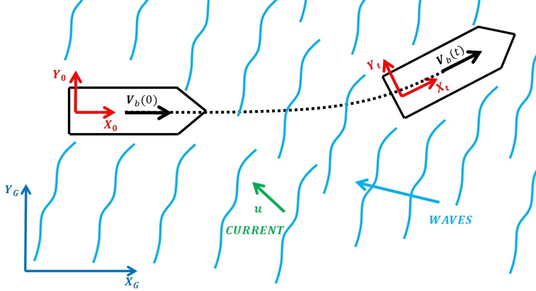
Based on the numerical approaches used in this work, it is convenient to solve Eqs. (4 21)-(4 25) in a frame of reference fixed to the moving body rather than on the global frame of reference. Therefore, the aforementioned equations will be solved in a local frame of reference. Figure 2 shows the global and local frame of reference. This frame of reference is assumed to match the global frame at time zero. For an observer sitting in the ship, the flow field around the ship will be \(\boldsymbol{U}_b (\boldsymbol{x}) = \boldsymbol{u} - \boldsymbol{V}_b (\boldsymbol{x})\). Therefore, the governing equations in the local frame of reference become:

(2.521)\[\begin{aligned} & \Delta \phi = 0 & \text{in } \Omega \end{aligned}\]

(2.522)\[\begin{aligned} & \frac{\partial \phi }{\partial t} + \boldsymbol{U}_b \cdot \nabla_h \phi + \frac{1}{2} \nabla_h \phi \cdot \nabla_h \phi + \nabla_h \psi \cdot \nabla_h \phi + \frac{P_{fs}}{\rho } + g\eta = 0 & \text{in } z = 0 \end{aligned}\]

(2.523)\[\begin{aligned} & \frac{\partial \eta }{\partial t} + \left( \boldsymbol{U}_b + \nabla_h \phi \right) \cdot \nabla_h \eta + \nabla_h \phi \cdot \nabla_h \zeta -\frac{\partial \phi }{\partial z} = 0 & \text{in } z = 0 \end{aligned}\]

(2.524)\[\begin{aligned} & \nabla_h \phi \cdot \boldsymbol{n}_p = -\left( \boldsymbol{v}_p + \boldsymbol{u} + \boldsymbol{v}_\psi \right) \cdot \boldsymbol{n}_p & \text{in } S_B \end{aligned}\]

(2.525)\[\begin{aligned} & \frac{\partial \phi }{\partial z} = 0 & \text{in } z = -H \end{aligned}\]

and the pressure induced by diffracted and radiated waves is:

(2.526)\[\begin{aligned} & P_p = -\rho \left( \frac{\partial \phi }{\partial t} + \left( \boldsymbol{U}_b + \nabla_h \phi + \nabla_h \psi \right) \cdot \nabla_h \phi -\frac{1}{2} \nabla \phi \cdot \nabla \phi \right) \end{aligned}\]

Fig. 2.19 Global and local frame of reference

where the incident wave potential and incident wave elevation must be transformed to the local frame of reference.

2.3.4.4. Flow linearization

The previous governing equations have been obtained under the assumption that \(\boldsymbol{v}_\phi \sim O(1)\). Then, the free surface boundary conditions can be written as follows:

(2.527)\[\begin{aligned} & \frac{\partial \phi }{\partial t} + \left( \boldsymbol{U}_b + \nabla_h \phi \right) \cdot \nabla_h \phi -\frac{1}{2} \nabla_h \phi \cdot \nabla_h \phi + \nabla_h \psi \cdot \nabla_h \phi + \frac{P_{fs}}{\rho } + g\eta = 0 & \text{in } z = 0 \end{aligned}\]

(2.528)\[\begin{aligned} & \frac{\partial \eta }{\partial t} + \left( \boldsymbol{U}_b + \nabla_h \phi \right) \cdot \nabla_h \eta + \nabla_h \phi \cdot \nabla_h \zeta -\frac{\partial \phi }{\partial z} = 0 & \text{in } z = 0 \end{aligned}\]

where \(\boldsymbol{U}_b + \nabla_h \phi\) represents the convective velocity. Since the convective velocity depends on \(\nabla_h \phi\), it must be updated every time step to account for variations of the convective velocity. While retaining this assumption allows for simulating transient flows, linearization of the convective velocity is a reasonable practice in many cases. While SeaFEM is capable of imposing the free surface boundary conditions without linearization at all, two commonly used linearizations are also available.

2.3.4.4.1. Neumann-Kelvin linearization

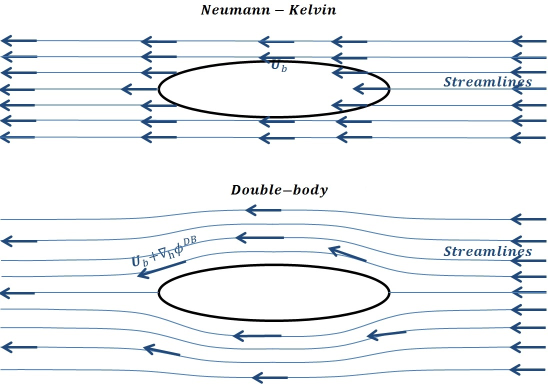
Neumann-Kelvin linearization assumes that \(\nabla_h \phi \sim O(\epsilon )\). This assumption is usually made for slender bodies whose perturbation of the flow field is small compared to the convective velocity. Then the convective velocity becomes the apparent velocity between the moving body and the water \(\boldsymbol{U}_b (\boldsymbol{x}) = \boldsymbol{u} - \boldsymbol{V}_b (\boldsymbol{x})\). Then the first order free surface boundary conditions become:

(2.529)\[\begin{aligned} & \frac{\partial \phi }{\partial t} + \boldsymbol{U}_b \cdot \nabla_h \phi + \frac{P_{fs}}{\rho } + g\eta = 0 & \text{in } z = 0 \end{aligned}\]

(2.530)\[\begin{aligned} & \frac{\partial \eta }{\partial t} + \boldsymbol{U}_b \cdot \nabla_h \eta -\frac{\partial \phi }{\partial z} = 0 & \text{in } z = 0 \end{aligned}\]

and the pressure induced by diffracted and radiated waves is:

(2.531)\[\begin{aligned} & P_p = -\rho \left( \frac{\partial \phi }{\partial t} + \boldsymbol{U}_b \cdot \nabla_h \phi \right) \end{aligned}\]

2.3.4.4.2. Double body linearization

Double body linearization assumes that \(\nabla_h \phi \sim O(1)\) but can be split into two terms: \(\nabla_h \phi = \nabla_h \phi^{DB} + \nabla_h \varphi^*\). \(\nabla_h \phi^{DB}\) represents the flow field when the free surface is substituted by a wall (equivalent to a symmetric case using a double body). Then \(\nabla_h \phi\) is approximately \(\nabla_h \phi^{DB}\), but perturbed by \(\nabla_h \phi^*\), which means \(\nabla_h \phi^{DB} \sim O(1)\) and \(\nabla_h \phi^* \sim O(\epsilon )\). Then the first order free surface boundary conditions become:

(2.532)\[\begin{split}\begin{aligned} & \frac{\partial \phi }{\partial t} + \left( \boldsymbol{U}_b + \nabla_h \phi^{DB} \right) \cdot \nabla_h \phi -\frac{1}{2} \nabla_h \phi^{DB} \nabla_h \phi^{DB} + \\ & + \nabla_h \phi^{DB} \cdot \nabla_h \psi + \frac{P_{fs}}{\rho } + g\eta = 0 & \text{in } z = 0 \end{aligned}\end{split}\]

(2.533)\[\begin{aligned} & \frac{\partial \eta }{\partial t} + \left( \boldsymbol{U}_b + \nabla_h \phi^{DB} \right) \cdot \nabla_h \eta + \nabla_h \phi^{DB} \cdot \nabla_h \zeta -\frac{\partial \phi }{\partial z} = 0 & \text{in } z = 0 \end{aligned}\]

and the pressure induced by diffracted and radiated waves is:

(2.534)\[\begin{aligned} & P_p = -\rho \left( \frac{\partial \phi }{\partial t} + \left( \boldsymbol{U}_b + \nabla_h \phi^{DB} \right) \cdot \nabla_h \phi -\frac{1}{2} \nabla_h \phi^{DB} \nabla_h \phi^{DB} + \nabla_h \phi^{DB} \cdot \nabla_h \psi \right) \end{aligned}\]

Free surface base flow based on Neumann-Kelvin (up) and double-body (down) linearization concepts

2.3.4.5. Transom stern boundary condition

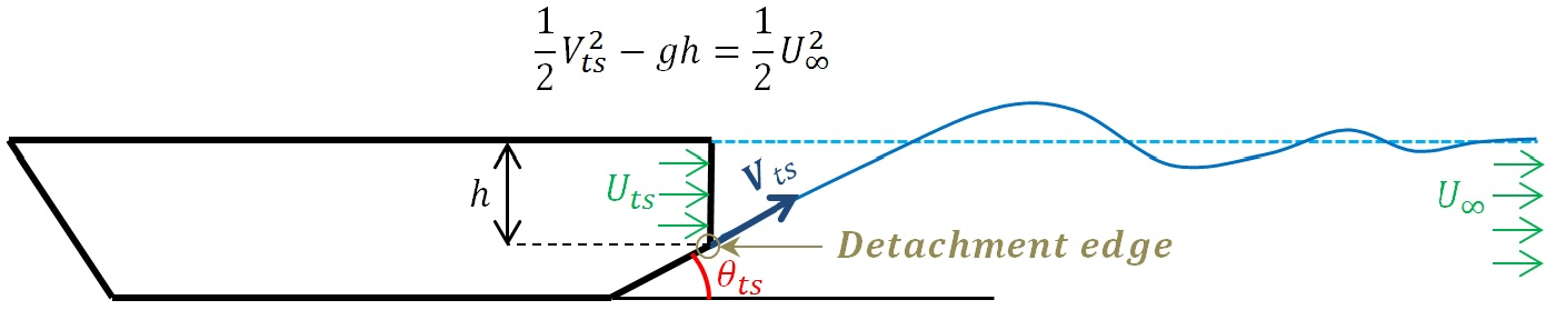
When considering moving bodies with transom sterns, flow detachment happens at the lower edge of the transom. While potential flow is incapable of predicting this sort of detachment, a transpiration model will be used to enforce it. To do so, the no flux body boundary condition is “not” used, on the contrary, a flux is allowed. The condition to be imposed is that streamlines departing from the detachment edge belong to the free surface. Then, the flux velocity is calculated based assuming that energy at the detachment edge is the same that the energy at the free surface far away downstream, where the free surface remains flat. Using Bernoulli’s equation, the flux velocity to be imposed is:

(2.535)\[\begin{split}\begin{aligned} & \frac{1}{2} \boldsymbol{V}_{ts}^2 - gh = \frac{1}{2} \boldsymbol{V}_\infty^2 \\ & U_{ts} = |\boldsymbol{V}_{ts} | cos⁡(\theta_ts )=\sqrt{(\boldsymbol{V}_\infty^2 + 2gh) } cos⁡(\theta_{ts} ) \end{aligned}\end{split}\]

Figure 4 explains the transpiration model implemented in SeaFEM.

Transpiration model for transom stern boundary condition with flow detachment