2.3.7. Body dynamics

2.3.7.1. Dynamic equations (small rotations)

Integrating the pressure over the bodies’ surface, the resulting forces and moments are obtained. On the other hand, the body dynamics is given by the equation of motion:

(2.581)\[\begin{aligned} & \overline{\overline{\boldsymbol{M}}} \boldsymbol{\ddot{X}} + \overline{\overline{\boldsymbol{K}}} \boldsymbol{X} = \boldsymbol{F} \end{aligned}\]

SeaFEM uses an implicit alpha modified Bossak-Newmark´s algorithm [2]:

(2.582)\[\begin{aligned} & \left( 1 - α \right) \boldsymbol{X}_{tt}^{n+1} + α \boldsymbol{X}_{tt}^n = \overline{\overline{\boldsymbol{M}}}^{-1} \left( \boldsymbol{F}^{n+1} - \overline{\overline{\boldsymbol{K}}} \boldsymbol{X}^{n+1} \right) \end{aligned}\]

(2.583)\[\begin{aligned} & \boldsymbol{X}_t^{n+1} = \boldsymbol{X}_t^n + ∆t \left[ \left(1-\Gamma \right)\boldsymbol{X}_{tt}^{n+1} + \Gamma \boldsymbol{X}_{tt}^n \right] \end{aligned}\]

(2.584)\[\begin{aligned} & \boldsymbol{X}^{n+1} = \boldsymbol{X}^n + ∆t \boldsymbol{X}_t^n + \frac{∆t^2}{2} \left[ \left(1-2β \right) \boldsymbol{X}_{tt}^{n+1} + 2β \boldsymbol{X}_{tt}^n \right] \end{aligned}\]

In the above integration algorithm, \(α\) is the parameter defining the numerical damping added in the integration. This damping creates a desirable stabilizing effect in the body dynamics integration. \(α\) is usually set to between \(0\) (no damping) and \(-0.1\). In SeaFEM, \(\Gamma ` and :math:`β\) are calculated as \(\Gamma = 0.5 - α\) and \(β = 0.5\Gamma + 0.025α\).

2.3.7.2. Dynamic equations (large rotations)

In case large rotations are expected, the Euler equations are used to integrate the body dynamics. Each body accelerations are solved respect to a local frame of reference attached to the gravity center of the body, and with axis parallel to the global frame of reference.

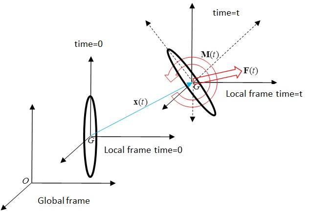
Fig. 2.21 Global and local frame of reference used in SeaFEM

The dynamic equations for each body are the Newton´s and Euler´s equations:

(2.585)\[\begin{aligned} & M_i \ddot{\boldsymbol{x}} = \boldsymbol{f}_i \end{aligned}\]

(2.586)\[\begin{aligned} & \overline{\overline{\boldsymbol{I}}}_i \ddot{\boldsymbol{r}}_i = \boldsymbol{m}_i - \dot{\boldsymbol{r}}_i ∧ \left( \overline{\overline{\boldsymbol{I}}}_i \cdot \dot{\boldsymbol{r}}_i \right) \end{aligned}\]

where \(\overline{\overline{\boldsymbol{I}}}_i ` is the instantaneous inertia tensor of body :math:`i\) respect to the local frame. The Euler equations are derived in a rotating reference frame fixed to the body, and therefore, the inertia has to be updated. It is important to remark that, in equation (7-6), \(\boldsymbol{F}\) and \(\boldsymbol{M}\) must be evaluated in the local reference frame.

2.3.7.3. Body links

2.3.7.3.1. Lagrange multipliers

Let a multibody system be defined by the dynamics equations:

(2.587)\[\begin{aligned} & \overline{\overline{\boldsymbol{M}}} \ddot{\boldsymbol{X}}^t = \boldsymbol{F}^t \end{aligned}\]

Let the body-links to be defined by nonlinear equations of the following type:

(2.588)\[\begin{aligned} & f_i \left( \boldsymbol{X}^t \right) = f_i \left(X_1^t, X_2^t, …, X_n^t \right) = b_i \end{aligned}\]

where \(x_j^t\) is the vector representing the position of all and each body of the multibody system, and \(b_i\) is a constant value. The latter will be brought into the system dynamics via Lagrange multipliers. To do so, body-links must be linearized. The following linearization is used:

(2.589)\[\begin{aligned} & f_i \left( X_1^{t,k}, X_2^{t,k}, …, X_n^{t,k} \right) + \sum_j \left( \frac{\partial f_i}{\partial x_j} \right)^{t,k} \left( X_j^{t,k+1} - X_j^{t,k} \right) = b_i \end{aligned}\]

in vector form:

(2.590)\[\begin{aligned} & \left(\nabla f_i \right)^{t,k} \cdot \boldsymbol{X}^{t,k+1} = b_i - f_i \left( \boldsymbol{X}^{t,k} \right) + \left(\nabla f_i \right)^{t,k} \cdot \boldsymbol{X}^{t,k} \end{aligned}\]

where \(k\) is the \(k-th\) iteration of the iterative resolution of the dynamic system. The previous linearization ensures that as \(‖\boldsymbol{X}^{t,k} - \boldsymbol{X}^({t,k+1} ‖ → 0 ⇒ f_i \left( \boldsymbol{X}^{t,k+1} \right) → b_i\) and the bodylink is fulfilled. We use an alpha Bossak-Newmark scheme as a temporal integrator scheme for the dynamic equations. Positions \(x_j^{t+∆t, k+1}\) depend linearly on accelerations \(\ddot{x}_j^{t+∆t, k+1}\) as follows:

(2.591)\[\begin{aligned} & \boldsymbol{X}^{t,k+1} = \boldsymbol{X}^{t-∆t} + ∆t \dot{\boldsymbol{X}} ̇^{t-∆t} + \frac{∆t^2}{2} \left( \left( 1-2β \right) \ddot{\boldsymbol{X}}^{t-∆t} + 2 β \ddot{\boldsymbol{X}}^{t,k+1} \right) \end{aligned}\]

Introducing the Newmark scheme into the linearized bodylink:

(2.592)\[\begin{split}\begin{aligned} & \left(\nabla f_i \right)^{t,k} \cdot \left( \boldsymbol{X}^{t-∆t} + ∆t \dot{X}^{t-∆t} + ∆t^2 \left( \left( 0.5-β \right) \ddot{\boldsymbol{X}} ^ {t,k+1} + β \ddot{\boldsymbol{X}} ^ {t-∆t} \right) \right) = \\ & = b_i - f_i \left( \boldsymbol{X}^{t,k} \right) + \left(\nabla f_i \right)^{t,k} \cdot \boldsymbol{X}^{t,k} \end{aligned}\end{split}\]

The previous equation can be written as:

(2.593)\[\begin{split}\begin{aligned} & \left(\nabla f_i \right)^{t,k} \cdot \ddot{\boldsymbol{X}}^{t,k+1} = \frac{1}{∆t^2 β} \left( b_i - f_i \left( \boldsymbol{X}^{t,k} \right) + \left(\nabla f_i \right)^{t,k} \cdot \boldsymbol{X}^{t,k} \right) - \\ & - \left(\nabla f_i \right)^{t,k} \cdot \left( \frac{X^{t-∆t}}{∆t^2 β} + frac{\dot{\boldsymbol{X}}^{t-∆t}}{∆t β} + \frac{(0.5-β)}{β} \ddot{\boldsymbol{X}}^{t-∆t} \right) \end{aligned}\end{split}\]

Or after reordering terms:

(2.594)\[\begin{aligned} & \left(\nabla f_i \right)^{t,k} \cdot \ddot{\boldsymbol{X}}^{t,k+1} = \frac{1}{∆t^2 β} \left(b_i - f_i \left(\boldsymbol{X}^{t,k} \right) \right) + \left(\nabla f_i \right)^{t,k} \cdot \ddot{\boldsymbol{X}}^{t,k} \end{aligned}\]

The set of linearized bodylinks can be written as:

(2.595)\[\begin{aligned} & \sum_j a_{ij}^{t,k} \ddot{X}_j^{t,k+1} = c_i^{t,k} \end{aligned}\]

where \(\overline{\overline{\boldsymbol{A}}}^{t,k} = \left[a_{ij}^{t,k} \right]\) is the Jacobian matrix

(2.596)\[\begin{aligned} & a_{ij}^{t,k} = \left( \frac{\partial f_i}{\partial x_j} \right)^{t,k} \end{aligned}\]

and \(\boldsymbol{c}^{t,k} = \left[ c_i^{t,k} \right]\):

(2.597)\[\begin{split}\begin{aligned} & c_i^{t,k} = \frac{1}{∆t^2 β} \left[ b_i - f_i \left(\boldsymbol{X}^{t,k} \right) + \sum_j a_{ij}^{t,k} X_j^{t,k} \right] \\ & - \sum_j a_{ij}^{t,k} \left( \frac{X_j^{t-∆t}}{∆t^2 β} + \frac{\dot{X}_j^{t-∆t}}{∆t β} + \frac{(0.5-β)}{β} \ddot{X}_j^{t-∆t} \right) \end{aligned}\end{split}\]

or

(2.598)\[\begin{aligned} & c_i^{t,k} = \frac{1}{∆t^2 β} \left[ b_i - f_i \left(x^{t,k} \right) \right]+\sum_j a_{ij}^{t,k} \ddot{X}_j^{t,k} \end{aligned}\]

Then, the imposition of nonlinear bodylinks via Lagrange multipliers can be carried out as follows:

(2.599)\[\begin{split}\begin{aligned} \begin{bmatrix} \overline{\overline{\boldsymbol{M}}} & \left( \overline{\overline{A}}^T \right)^{t,k} \\ \overline{\overline{A}}^{t,k} & 0 \\ \end{bmatrix} \begin{bmatrix} \ddot{x}^{t,k+1} \\ \lambda^{t,k+1} \\ \end{bmatrix} = \begin{bmatrix} \boldsymbol{F}^{t,k} \\ \boldsymbol{c}^{t,k} \end{bmatrix} \end{aligned}\end{split}\]

Finally, reaction forces are obtained from:

(2.600)\[\begin{aligned} & \boldsymbol{R}^{t,k} = - \left( \overline{\overline{A}}^T \right)^{t,k} \lambda^{t,k} \end{aligned}\]

and since matrix contains the instantaneous normal direction to the trajectory imposed by the body-links, reaction forces act perpendicular to the imposed trajectories.

2.3.7.3.2. Body links with Alpha Bossak-Newmark integration

The alpha Bossak-Newmark scheme uses the following scheme to obtain the acceleration at time t:

(2.601)\[\begin{aligned} & (1-α) \overline{\overline{\boldsymbol{M}}} \ddot{\boldsymbol{X}}^t + α \overline{\overline{\boldsymbol{M}}} \ddot{\boldsymbol{X}}^{t-\Delta t} = \boldsymbol{F}^t + \boldsymbol{R}^t \end{aligned}\]

where \(\boldsymbol{R}^t = - \overline{\overline{A}}^T \lambda^t\) are the reaction forces due to bodylinks. Then:

(2.602)\[\begin{aligned} & \overline{\overline{\boldsymbol{M}}} (1-α) \ddot{\boldsymbol{x}}^t + \overline{\overline{\boldsymbol{A}}}^T \lambda^t = \boldsymbol{F}^t - α \boldsymbol{M} \ddot{\boldsymbol{x}}^{t-\Delta t} \end{aligned}\]

Introducing the body link constraints \(\boldsymbol{A} \ddot{\boldsymbol{x}}^t = \boldsymbol{c}^t\), the multibody dynamic system reads as:

(2.603)\[\begin{split}\begin{aligned} \begin{bmatrix} \overline{\overline{\boldsymbol{M}}} & \overline{\overline{\boldsymbol{A}}}^T \\ \overline{\overline{\boldsymbol{A}}} & 0 \\ \end{bmatrix} \begin{bmatrix} (1-\alpha) \ddot{\boldsymbol{x}}^t \\ \lambda^t \\ \end{bmatrix} = \begin{bmatrix} \boldsymbol{F}^t - \alpha \overline{\overline{\boldsymbol{M}}} \ddot{\boldsymbol{x}}^{t - \Delta t} \\ (1-\alpha) \boldsymbol{c}^t \end{bmatrix} \end{aligned}\end{split}\]

2.3.7.4. Body dynamics iterative solver

The dynamic solver is implemented in SeaFEM by means of three nested loops. A relaxation algorithm based on the Aitken´s method [6] is used to speed up convergence within each loop.

2.3.7.4.1. Time marching loop

The time marching loop is the outer loop marching in time. Information from the previous time step is used as initial guests of the iterative procedure.

2.3.7.4.2. Solver loop

The solver loop is where the hydrodynamic loads are calculated. In each iteration within this loop, the linear system corresponding to the wave diffraction-radiation problem is to be solved. Iterations is carried out until convergence of hydrodynamic loads along with body kinematics is reached. Should non-linear mooring lines be defined, stiffness linearization will be carried out for each iteration, and the updated stiffness matrix will be passed on to the body dynamics loop.

2.3.7.4.3. Body dynamics loop

The body dynamics loop is the inner loop. Within this loop, wave diffraction and radiation loads remain unchanged, hydrostatic forces are updated based on body position, and the rest of loads will be updated in each iteration.

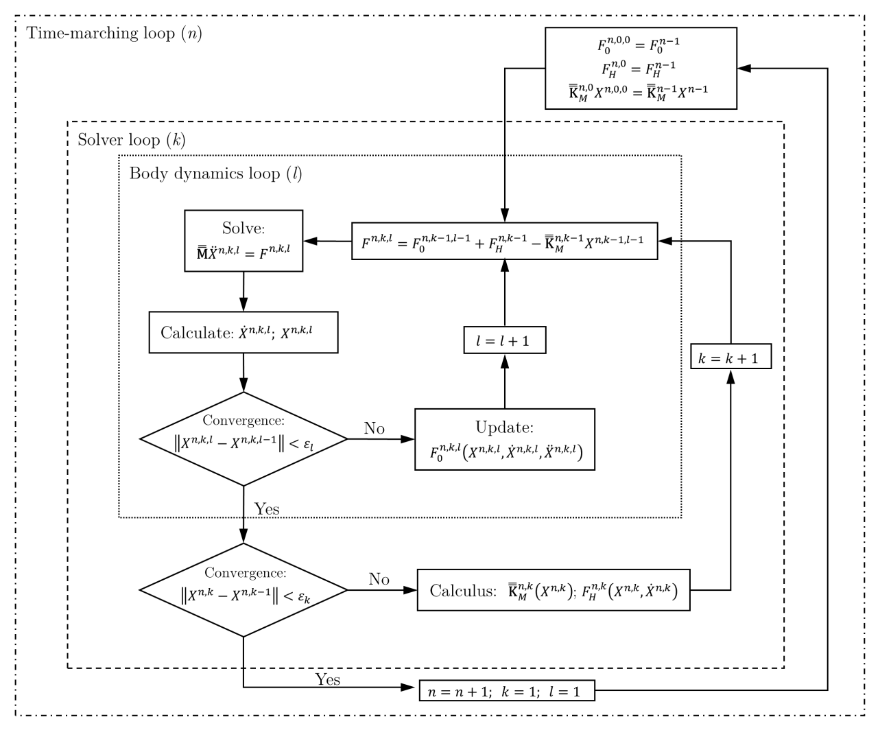
Fig. 2.22 Scheme of the dynamic integration solver of SeaFEM