2.3.12. Solver acceleration
2.3.12.1. Introduction
Most of the computational effort of the proposed numerical algorithm is spent in solving the linear system resulting from the wave diffraction-radiation problem. Therefore, our main focused in order to reduce the computational time is speeding up the linear solver. To do so, two techniques, that can be used combined, have been analyzed: the use of deflated solver, and the use of parallel computing in graphic processing units.
2.3.12.2. Solver deflation
Deflation works by considering piecewise constant approximations on coarse sub-domains. These piecewise constant approximations are associated to the low frequencies eigenmodes of the solution, which are also the slow convergence modes [ , ]. Then, these slow modes can be quickly approximated by solving a smaller linear system of equations that can be incorporated to the traditional preconditioned iterative solvers in order to accelerate the convergence of the solution. Hence, the use of preconditioning technique is compatible with the use of preconditioners. The first step is to divide the domain into a set of coarse sub-domains capable of capturing the slow modes. Several techniques have been developed for this purpose [ , ]. Some authors has proposed a technique based on using seed-points to start building the sub-domains, and sub-domains are created by associating nodes to their closer seeds [15]. This technique has the disadvantage of requiring prescribing the seeds. The algorithm developed for SeaFEM [1] is based on level structure criteria, where nodes are associated to a central node based on the level structure rooted at this central node (concept from graph theory). A maximum level structure “L”, where L refers to the neighbouring level respect to the central node, is prescribed. Figure 10 shows a domain decomposition obtained using this level structure technique with level L=2. Ordered pair (sub-domain, level) is used to identify nodes and sub-domains they belong to, and their corresponding structure level. Notice that nodes will accept to belong to a new sub-domain, if and only if its structure level in that sub-domain is lower than its level in its current sub-domain. The algorithm used to obtain such decomposition is presented step by step next:
Step 0: Assigned level L+1 to all nodes
Step 1: Start building sub-domain 0: offer level 0 to the first node of the mesh (root node for sub-domain 0). It will become node (sub-domain, level)=(0,0)
Step 2: Identify neighbours of the root node (node (0,0)) and offer them level 1: nodes (0,1)
Step 3: Identify neighbours of nodes (0,1), and offer them level 2: nodes (0,2)
Step 4: The procedure is repeated until the prescribed level “L” is reached
Step 5: The first node still with level L+1 (based on the numbering of the nodes) is used as root node for sub-domain 1, and it is given level 0, becoming the root node (1,0)
Step 6: Identify neighbours of the root node (1,0) and offer them level 1: nodes (1,1) (Notice that some (0,L) nodes might become (1,1))
Step 7: Identify neighbours of nodes (1,1), and offer them level 2: nodes (1,2). (Notice that some (0,L) or (0,L-1) nodes might become (1,2) if L>2 or L-1>2 respectively)
Step 8: The procedure is repeated until the nodes (1,L) are identified
Step 9: Repeat Steps 5-8 until there is no node with level L+1
This algorithm guarantees that any node cannot have a lower structure level respect to any other root node. And the higher the prescribed level, the lower the number of sub-domains created. Although the previous algorithm provides good results, it can be improved by using it twice. In a first round, rather than using the prescribed level L, a structure level 2L is used instead. Then a first decomposition is found with a lower number of sub-domains and twice the maximum structure level. In a second round, the procedure is repeated with a maximum structure level L and using as root those nodes with higher levels. Figure 11 shows the sub-domain decomposition obtained using the two rounds technique. The first one shows the decomposition after the first round at level 2L, and the second shows the decomposition after the second round at level L starting of the first decomposition at level 2L. Notice that the level at the sub-domains boundaries is lower or equal than the prescribed level L, and always minimum respect to any central node (node of level zero). The recommended number of sub-domains might depend on the specific case under study. Usually in the order of hundred is a recommended value. In our specific case, the matrix of the linear system to be solved remains the same during the calculation, so that the sub-domain decompositions have to be carried out just once. The deflated system has to be solved every iteration of the solver. However, since in our case study the linear system of equation to be solved remains the same along the simulation, so does the deflated matrix. The inverse of the deflated matrix can be calculated just in the first time step, and then be stored. Hence, the resolution of the deflated system within each iteration can be substituted by a matrix vector multiplication.
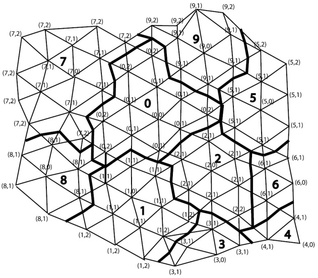
Fig. 2.24 Sub-domain decomposition using the neighboring level algorithm
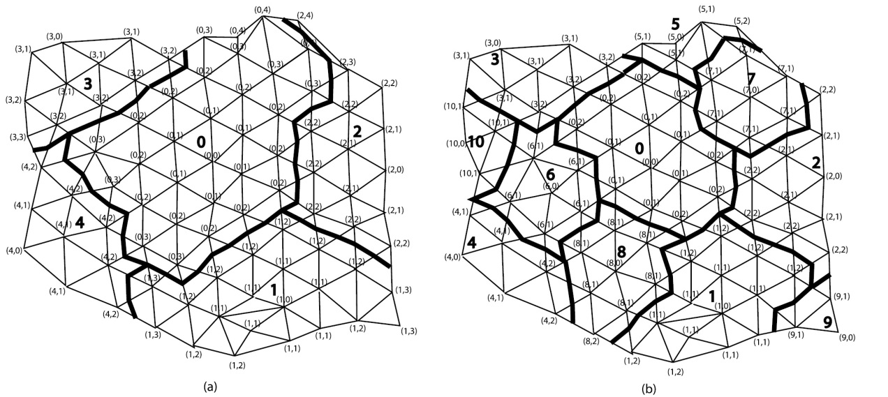
Fig. 2.25 Sub-domain decomposition using the two-rounds neighboring level algorithm. (a) Decomposition after first round. (b) Decomposition after second round
2.3.12.3. Solver GPU acceleration
The fast development of the videogame industry is leading to higher computational capabilities of GPUs. Hence, their use for heavy computations in computational fluid dynamics is becoming more common (see [ , ]). The implementation carried out in SeaFEM [1] is based on the well-known CUDA, a parallel computing platform and programming model invented by NVIDIA. It is focussed in speeding up the iterative solver using the functions provided by the cublas and cusparse libraries. Deflated and non-deflated preconditioned conjugate gradient (CG) algorithm has been implemented in CUDA, along with a sparse approximate inverse (SPAI) preconditioner [ ] and incomplete LU decomposition (ILU) preconditioner. However, using the sparse lower and upper triangular solvers provided in the cusparse library for ILU preconditioning resulted in poor performance. This poor performance can be expected since solving triangular system are not suitable for massive parallelization across tens of thousands threads [19], as required by GPUs in order to hide memory latency. Therefore we will omit the use of the ILU preconditioner when reporting GPU results. Since the system matrix remains the same along the computation, preconditioners are calculated just once and in the first time step. Then, computational time invested in calculating preconditioners is negligible when compared to the total time spent in the linear solver during the whole simulation.
2.3.12.4. CPU Direct solver
SeaFEM has available a direct solver to be used with CPUs. It is advised to use this solver in those cases where the system matrix remains the same along the simulation. If the system matrix needs to be updated as the simulation advances, the direct solver will be slower when compared to iterative solvers.
2.3.12.5. OpenMP parallelization
OpenMP has been used for parallelization of CPU solvers as well as for evaluating analytical formulas. For instance, when evaluating irregular seas modelled by spectra discretization based on Airy waves, a large number of waves might be used, thus requiring a significant CPU time compared to the solver CPU time. Open MP has been used in SeaFEM to reduce the CPU time of this type of computations.