2.3.1. Mathematical model for wave problems (Part I)

2.3.1.1. Governing equations

2.3.1.1.1. Flow equation and boundary conditions

Assuming incompressible flow \((\nabla \cdot \boldsymbol{v})\) and irrotational flow \((\nabla \times \boldsymbol{v}_\phi = 0 \Rightarrow \boldsymbol{v}_\phi = \nabla \phi)\), then the flow governing equations are given by:

(2.380)\[\begin{align} & \Delta \varphi = 0 & \text{in } \Omega \end{align}\]

(2.381)\[\begin{split}\begin{align} & \frac{\partial \xi }{\partial t} + \frac{\partial \varphi}{\partial x} \frac{\partial \xi }{\partial x} + \frac{\partial \varphi}{\partial y} \frac{\partial \xi }{\partial y} - \frac{\partial \varphi}{\partial z} = 0 & \text{on } z = \zeta \\ \end{align}\end{split}\]

(2.382)\[\begin{split}\begin{align} & \frac{\partial \varphi}{\partial t} + \frac{1}{2} \nabla \varphi \cdot \nabla \varphi + \frac{P_{fs}}{\rho } + g\xi = 0 & \text{on } z = \zeta \\ \end{align}\end{split}\]

(2.383)\[\begin{split}\begin{align} & \boldsymbol{v}_p \cdot \boldsymbol{n}_p + \boldsymbol{v}_\phi \cdot \boldsymbol{n}_p = 0 & \text{on } S_B \\ \end{align}\end{split}\]

(2.384)\[\begin{align} & P_p= -\rho \frac{\partial \varphi}{\partial t} -\frac{1}{2} \rho \nabla \varphi \cdot \nabla \varphi - \rho gz_p & \text{in } \Omega \end{align}\]

2.3.1.1.2. Solution approach

Taylor series expansion

Free surface and body boundary condition (BC) will be applied on \(z=0\). Taylor series expansion are carried out to both free surface BCs around \(z=0\) to approximate the BC on \(z=\zeta\). Body boundary condition will be applied on \(S_B^0\). Taylor series expansion are carried out around \(S_B^0\) to approximate the BC on \(S_B\).

Perturbed solution

A perturbed solution based on stokes waves approximation is used, where the velocity potential and free surface elevation are perturbed as:

(2.385)\[\begin{aligned} & \varphi = \epsilon^1\varphi^1 + \epsilon^2\varphi^2 + \epsilon^3\varphi^3 + ... \end{aligned}\]

(2.386)\[\begin{aligned} & \xi = \epsilon^1\xi^1 + \epsilon^2\xi^2 + \epsilon^3\xi^3 + ... \end{aligned}\]

Body movement solution is also assumed to be a perturbed solution:

(2.387)\[\begin{aligned} & \boldsymbol{X} = \epsilon^1\boldsymbol{X} ^1 + \epsilon^2\boldsymbol{X}^2 + \epsilon^3\boldsymbol{X}^3 + ... \end{aligned}\]

(2.388)\[\begin{aligned} & \boldsymbol{V} = \epsilon^1\boldsymbol{V}^1 + \epsilon^2\boldsymbol{V}^2 + \epsilon^3\boldsymbol{V}^3 + ... \end{aligned}\]

Then the translational vector of any point P on the body surface can be perturbed as:

(2.389)\[\begin{aligned} & \boldsymbol{r}_p = \epsilon^1\boldsymbol{r}_p^1 + \epsilon^2\boldsymbol{r}_p^2 + \epsilon^3\boldsymbol{r}_p^3 + ... \end{aligned}\]

where

(2.390)\[\begin{aligned} & \boldsymbol{X}^i = (\delta_x^i, \delta_y^i, \delta_z^i, \theta_x^i, \theta_y^i, \theta_z^i) = (\boldsymbol{\delta}^i, \boldsymbol{\theta}^i) \end{aligned}\]

(2.391)\[\begin{aligned} \boldsymbol{r}_p^1 = \boldsymbol{\delta}^1 + \boldsymbol{\theta}^1 \times \overrightarrow{\boldsymbol{R^0P^0}} \end{aligned}\]

(2.392)\[\begin{aligned} \boldsymbol{r}_p^{1+2} = \boldsymbol{\delta}^{1+2} + \boldsymbol{\theta}^{1+2} \times \overrightarrow{\boldsymbol{R^0P^0}} + \boldsymbol{\overline{\overline{H}}} \overrightarrow{\boldsymbol{R^0P^0}} \end{aligned}\]

(2.393)\[\begin{split}\begin{aligned} \boldsymbol{\overline{\overline{H}}} = \frac{1}{2} \begin{pmatrix} -(\theta_y^2 + \theta_z^2) & 0 & 0 \\ 2\theta_x\theta_y & -(\theta_x^2 + \theta_z^2) & 0 \\ 2\theta_x\theta_z & 2\theta_y\theta_z & -(\theta_x^2 + \theta_y^2) \end{pmatrix} \end{aligned}\end{split}\]

(2.394)\[\begin{aligned} \boldsymbol{V}^i = (v_x^i, v_y^i, v_z^i, \omega_x^i, \omega_y^i, \omega_z^i) = (\boldsymbol{v}^i, \boldsymbol{\omega}^i) \end{aligned}\]

(2.395)\[\begin{aligned} \boldsymbol{v}_p^1 = \boldsymbol{v}^1 + \boldsymbol{\omega}^1 \times \overrightarrow{\boldsymbol{R^0P^0}} \end{aligned}\]

(2.396)\[\begin{aligned} \boldsymbol{v}_p^{1+2} = \boldsymbol{v}^{1+2} + \boldsymbol{\omega}^{1+2} \times \overrightarrow{\boldsymbol{R^0P^0}} + \dot{\boldsymbol{\overline{\overline{H}}}} \overrightarrow{\boldsymbol{R^0P^0}} \end{aligned}\]

(2.397)\[\begin{aligned} \boldsymbol{n}_p^1 = \boldsymbol{n}_p^0 + \boldsymbol{\theta}^1 \times \boldsymbol{n}_p^0 \end{aligned}\]

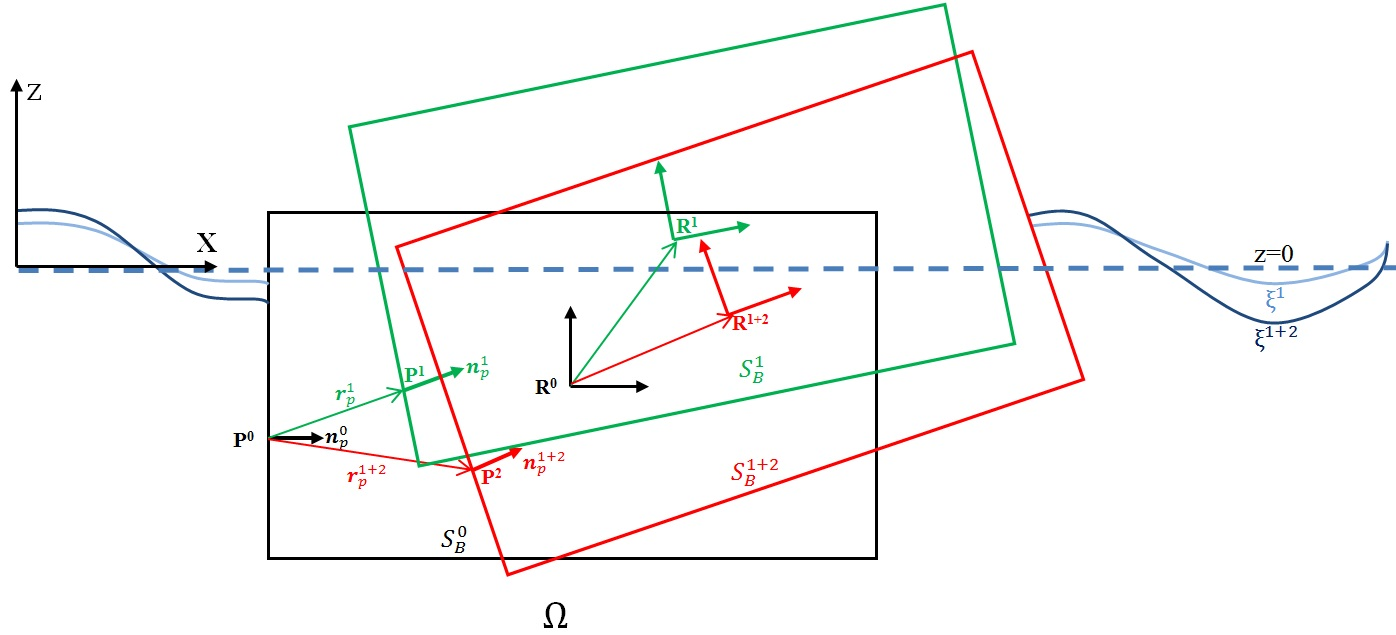
Fig. 2.18 First and second order rigid body movements

2.3.1.2. First order approach

2.3.1.2.1. First order governing equations

After carrying out the Taylor series expansions, using the perturbed solution, and retaining terms of order \(\epsilon\), the first order governing equations become:

(2.398)\[\begin{align} & \Delta \varphi^1=0 & \text{in } \Omega \end{align}\]

(2.399)\[\begin{split}\begin{align} & \frac{\partial \xi^1}{\partial t} - \frac{\partial \varphi^1}{\partial z} = 0 & \text{in } z = 0 \\ \end{align}\end{split}\]

(2.400)\[\begin{split}\begin{align} & \frac{\partial \varphi^1}{\partial t} \frac{P_{fs}}{\rho } + g\xi^1 = 0 & \text{in } z = 0 \\ \end{align}\end{split}\]

(2.401)\[\begin{split}\begin{align} & \boldsymbol{v}_p^1 \cdot \boldsymbol{n}_p^0 + \boldsymbol{v}_\phi^1 \cdot \boldsymbol{n}_p^0 = 0 & \text{in } S_B \\ \end{align}\end{split}\]

and the first order pressure at a point \(P_p^1\) on the body surface is

(2.402)\[\begin{aligned} & P_p^1 = P_H^0 + P_H^1 + P_D^1 & \text{in } \boldsymbol{S_B} \end{aligned}\]

where \(P_D^1=-\rho (\partial \varphi^1 )/\partial t, P_H^0=-\rho gz_p\), and \(P_H^1=-\rho gr_{pz}^1\).

2.3.1.2.2. First order decomposition solution

The total velocity potential can be decomposed as:

(2.403)\[\begin{aligned} \varphi^1 = \psi^1 + \phi^1 \end{aligned}\]

(2.404)\[\begin{aligned} \xi^1 = \zeta^1 + \eta^1 \end{aligned}\]

where \(\psi^1\) is the incident wave potential, and \(\phi\) is the diffraction-radiation wave potential.

First-order incident wave solution

The incident wave velocity potential \(\psi^1\) fulfils the following equations:

(2.405)\[\begin{aligned} & \nabla \psi^1 = 0 & \text{in } \Omega \end{aligned}\]

(2.406)\[\begin{aligned} & \frac{\partial \zeta^1}{\partial t} - \frac{\partial \psi^1}{\partial z} = 0 & \text{in } z = 0 \end{aligned}\]

(2.407)\[\begin{aligned} & \frac{\partial \psi^1}{\partial t} + g\zeta^1 = 0 & \text{in } z = 0 \end{aligned}\]

(2.408)\[\begin{aligned} & \frac{\partial \psi^1}{\partial z} = 0 & \text{in } z = -H \end{aligned}\]

Eqs. eq:incident1 - eq:incident4 have an analytical solution, known as the Airy wave solution:

(2.409)\[\begin{split}\begin{aligned} & \psi^1=\sum_i \frac{A_i g}{\omega_i} \frac{cosh⁡(|\boldsymbol{k}_i |(H+z))}{cosh⁡(|\boldsymbol{k}_i |H)} sin⁡(\boldsymbol{k}_i \boldsymbol{x} - \omega_i t+\alpha_i) \\ & \zeta^1=\sum_i A_i cos⁡(\boldsymbol{k}_i \boldsymbol{x} - \omega_i t+\alpha_i) \end{aligned}\end{split}\]

where \(A\) is the wave amplitude, \(H\) is a constant water depth, \(\boldsymbol{k}=2π/L (cos⁡(\Gamma ),sin⁡(\Gamma ) )\), \(L\) is the wave length, \(\Gamma ` is the wave propagation direction, :math:\)omega=2π/T`, \(T\) is the wave period, and \(\alpha\) is the wave phase delay. The following dispersion relation holds:

(2.410)\[\begin{aligned} \omega_i^2 = g|\boldsymbol{k}_i | tanh⁡(|\boldsymbol{k}_i |H) \end{aligned}\]

and the fluid pressure induced by the Airy wave in a point \(P\) is given by:

(2.411)\[\begin{aligned} P_p\psi^1=\sum_i \rho gA_i cosh⁡(|\boldsymbol{k}_i |(H+z))/cosh⁡(|\boldsymbol{k}_i |H) cos (\boldsymbol{k}_i \boldsymbol{x} - \omega_i t+\alpha_i) \end{aligned}\]

In the asymptotic case of infinite water depth \((H→\infty )\), the factor \(cosh⁡(|\boldsymbol{k}|(H+z))/cosh⁡(|\boldsymbol{k}|H) →exp⁡(|\boldsymbol{k}|z)\).

First-order diffraction-radiation wave problem

The governing equations for the diffraction-radiation velocity potential \(\phi^1\) is given by:

(2.412)\[\begin{aligned} & \Delta \phi^1=0 & \text{in } \Omega \end{aligned}\]

(2.413)\[\begin{aligned} & \frac{\partial \eta^1}{\partial t} - \frac{\partial \phi^1}{\partial z} = 0 & \text{on } z=0 \end{aligned}\]

(2.414)\[\begin{aligned} & \frac{\partial \phi^1}{\partial t} + \frac{P_{fs}}{\rho } + g\eta^1 = 0 & \text{on } z=0 \end{aligned}\]

(2.415)\[\begin{aligned} & \boldsymbol{v}_\phi^1 \cdot \boldsymbol{n}_p^0 = -\boldsymbol{v}_p^1 \cdot \boldsymbol{n}_p^0 - \boldsymbol{v}_\psi^1 \cdot \boldsymbol{n}_p^0 & \text{on } P \in S_B \end{aligned}\]

and the fluid pressure at a point \(P\) on the body surface is given by:

(2.416)\[\begin{aligned} & P_p^1 = P_{ph}^0 + P_{ph}^1 + P_{p\psi}^1 + P_{p\phi}^1 & \text{on } P \in S_B \end{aligned}\]

where \(P_{p\phi}^1 = -\rho (\partial \phi^1)/\partial t\), \(P_{ph}^0 = -\rho gz\), and \(P_{ph}^1 = -\rho gr_{pz}^1\).

2.3.1.3. Second order approach

2.3.1.3.1. Second-order governing equations

After carrying out the Taylor series expansions, using the perturbed solution, and retaining terms up to order \(\epsilon^2\), and considering that \(\varphi^{1+2}=\varphi^1+\varphi^2\), \(\xi^{1+2}=\xi^1+\xi^2\) , \(P_p^{1+2}=P_p^1+P_p^2\), \(X_B^{1+2}=X_B^1+X_B^2\), \(V_B^{1+2}=V_B^1+V_B^2\), \(v_p^{1+2}=v_p^1+v_p^2\), \(v_\phi^{1+2}=v_\phi^1+v_\phi^2, r_p^{1+2}=r_p^1+r_p^2\), the governing equations become:

(2.417)\[\begin{aligned} & \Delta \varphi^{1+2}=0 & \text{in } \omega \end{aligned}\]

(2.418)\[\begin{aligned} & \frac{\partial \xi^{1+2}}{\partial t} - \frac{\partial \varphi^{1+2}}{\partial z} = \xi^1 \frac{\partial}{\partial z} \left(\frac{\partial \varphi^1}{\partial z}\right) - \frac{\partial \xi^1}{\partial x} \frac{\partial \varphi^1}{\partial x} - \frac{\partial \xi^1}{\partial y} \frac{\partial \varphi^1}{\partial y} & \text{in } z=0 \end{aligned}\]

(2.419)\[\begin{aligned} & \frac{\partial \varphi^{1+2}}{\partial t} + \frac{P_{fs} }{\rho } + g\xi^{1+2} = -\xi^1 \frac{\partial}{\partial z} \left(\frac{\partial \varphi^1}{\partial t}\right) -\frac{1}{2} \nabla \varphi^1 \cdot \nabla \varphi^1 & \text{in } z=0 \end{aligned}\]

(2.420)\[\begin{aligned} & (\boldsymbol{v}_p^1 + \boldsymbol{v}_\phi^1 ) \cdot \boldsymbol{n}_p^1 + (\boldsymbol{v}_p^2 + \boldsymbol{v}_\phi^2)\cdot \boldsymbol{n}_p^0 = -(\boldsymbol{r}_p^1 \cdot \nabla \boldsymbol{v}_\phi^1) \cdot \boldsymbol{n}_p^0 & \text{in } S_B^0 \end{aligned}\]

and the pressure at a point \(P\) on the body surface is:

(2.421)\[\begin{aligned} & P_p^{1+2} = P_H^0+P_H^{1+2}+P_D^{1+2} & in S_B^0 \end{aligned}\]

where \(P_H^0=-\rho gz_p\), and \(P_H^{1+2} = -\rho gr_{pz}^{1+2}\), and \(P_D^{1+2} = -\rho (\partial \varphi^{1+2})/\partial t-\rho r_p^1 \cdot \nabla ((\partial \varphi^1)/\partial t)-\rho 1/2 \nabla \varphi^1 \cdot \nabla \varphi^1\).

2.3.1.3.2. Second-order decomposition solution

Second-order incident wave solution

The second-order total velocity potential can be decomposed as:

(2.422)\[\begin{aligned} \varphi^2=\psi^2+\phi^2 \end{aligned}\]

(2.423)\[\begin{aligned} \xi^2=\zeta^2+\eta^2 \end{aligned}\]

where \(\psi^2\) is the second-order incident wave potential, and \(\phi^2\) is the second-order diffraction-radiation wave velocity potential. The up to second-order incident wave potential and free surface elevation fulfils the following equations:

\[\begin{aligned} & \Delta \psi^{1+2}=0 & \text{in } \Omega \end{aligned} :label:2ndOrderGovEquations1\]

\[\begin{aligned} & \frac{\partial \zeta^{1+2}}{\partial t} - \frac{\partial \psi^{1+2}}{\partial z} = \zeta^1 \frac{\partial ^2 \psi^1}{\partial z^2} - \frac{\partial \zeta^1}{\partial x} \frac{\partial \psi^1}{\partial x} - \frac{\partial \zeta^1}{\partial y} \frac{\partial \psi^1}{\partial y} & \text{on } z=0 \end{aligned} :label:2ndOrderGovEquations2\]

\[\begin{aligned} & \frac{\partial \psi^{1+2}}{\partial t} + g\zeta^{1+2} = -\zeta^1 \frac{\partial }{\partial z} \left(\frac{\partial \psi^1}{\partial t}\right) - \frac{1}{2} \nabla \psi^1 \cdot \nabla \psi^1 & \text{on } z=0 \end{aligned} :label:2ndOrderGovEquations3\]

\[\begin{aligned} & \frac{\partial \psi^{1+2}}{\partial z}=0 & \text{on } z=-H \end{aligned} :label:2ndOrderGovEquations4\]

The solution to eq:2ndOrderGovEquations1 - eq:2ndOrderGovEquations4 is as follows:

(2.424)\[\begin{split}\begin{aligned} \psi^{1+2} = \psi^1 + \sum_i B_{ij}^0 sin (2 (\boldsymbol{k_i} \boldsymbol{x} - \omega_i t + \alpha_i )) \\ + \sum_{j>i} \sum_i B_{ij}^+ cosh⁡ (|\boldsymbol{k}_i + \boldsymbol{k}_j| (H+z)) sin ((\boldsymbol{k}_i \boldsymbol{x} - \omega_i t + \delta_i) + (\boldsymbol{k}_j \boldsymbol{x} - \omega_j t + \alpha_j )) \\ + \sum_{j>i} \sum_i B_{ij}^- cosh⁡ (|\boldsymbol{k}_i - \boldsymbol{k}_j |(H+z)) sin ((\boldsymbol{k}_i \boldsymbol{x} - \omega_i t + \delta_i ) - (\boldsymbol{k}_j \boldsymbol{x} - \omega_j t + \alpha_j )) \end{aligned}\end{split}\]

where the coefficients are given in table 1. In the asymptotic case of infinite depth \((H→\infty )\) the coefficients \(B_{ij}^0→0\) , \(D_{ij}^+→\infty `, :math:`D_{ij3}^-→\infty `, :math:`B_{ij}^+→0\), \(B_{ij}^-→0\). Then, the second order velocity potential becomes null. The wave elevation up to second order is obtained from:

(2.425)\[\begin{aligned} \zeta^{1+2} = -\frac{1}{g} \left(\frac{\partial\psi^{1+2}}{\partial t} + \frac{P}{\rho } + \zeta^1 \frac{\partial}{\partial z} \left(\frac{\partial \psi^1}{\partial t}\right) + \frac{1}{2} \nabla \psi^1 \cdot \nabla \psi^1 - C^1\right) \end{aligned}\]

and the fluid pressure induced by the second order wave potential at a point \(P\) is:

(2.426)\[\begin{aligned} P_{p\psi}^{1+2} = - \rho \left(\frac{\partial \psi^{1+2}}{\partial t} + \frac{1}{2} \nabla \psi^1 \cdot \nabla \psi^1\right) - \rho \left(\boldsymbol{r}_p^1 \cdot \nabla \left(\frac{\partial \psi^1}{\partial t}\right)\right) \end{aligned}\]

In the asymptotic case of infinite depth \((H→\infty )\) the coefficients \(B_{ij}^0→0\) , \(D_{ij}^+→\infty `, :math:`D_{ij3}^-→\infty `, :math:`B_{ij}^+→0\), \(B_{ij}^-→0\). Then, the second order velocity potential becomes null.

(2.427)\[\begin{split}\begin{aligned} & B_{ij}^0 = \frac{3A_i^2 g|\boldsymbol{k}_i |}{8 \omega_i} \frac{cosh⁡(2|\boldsymbol{k}_i |(H+z))}{sinh^3⁡(|\boldsymbol{k}_i |H) cosh⁡(|\boldsymbol{k}_i |H)} \\ & B_{ij}^+ = \frac{\sum_{k=1}^3 C_{ijk}^+}{D_{ijk}^+} \\ & B_{ij}^- = \frac{\sum_(k=1)^3 C_{ijk}^-}{D_{ijk}^-} \\ & C_{ij1}^+ = \frac{A_i A_j}{2g} \omega_i^2 (\omega_i + \omega_j) \\ & C_{ij1}^- = \frac{A_i A_j}{2g} \omega_i^2 (\omega_i - \omega_j) \\ & C_{ij2}^+ = \frac{A_i A_j}{4g} (\omega_i \omega_j - g^2 \frac{\boldsymbol{k}_i \cdot \boldsymbol{k}_j}{\omega_i \omega_j})(\omega_i+\omega_j) \\ & C_{ij2}^- = - \frac{A_i A_j}{4g} (\omega_i \omega_j + g^2 \frac{\boldsymbol{k}_i \cdot \boldsymbol{k}_j}{\omega_i \omega_j})(\omega_i-\omega_j) \\ & C_{ij3}^+ = - \frac{A_i A_j}{2} \frac{g}{\omega_i} (|\boldsymbol{k}_i|^2 + \boldsymbol{k}_i \cdot \boldsymbol{k}_j) \\ & C_{ij3}^- = \frac{A_i A_j}{2} \frac{g}{\omega_i} (|\boldsymbol{k}_i|^2 - \boldsymbol{k}_i \cdot \boldsymbol{k}_j) \\ & D_{ij}^+ = |\boldsymbol{k}_i + \boldsymbol{k}_j| sinh(|\boldsymbol{k}_i + \boldsymbol{k}_j| H) -\frac{1}{g} (\omega_i + \omega_j)^2 cosh⁡(|\boldsymbol{k}_i + \boldsymbol{k}_j| H) \\ & D_{ij3}^- = |\boldsymbol{k}_i - \boldsymbol{k}_j| sinh(|\boldsymbol{k}_i - \boldsymbol{k}_j| H) -\frac{1}{g} (\omega_i - \omega_j)^2 cosh⁡(|\boldsymbol{k}_i + \boldsymbol{k}_j| H) \end{aligned}\end{split}\]

Table 1 Stoke´s second-order wave potential coefficients

Second-order diffraction-radiation wave problem

The governing equations for the diffraction-radiation velocity potential up to second-order \(\phi^{1+2}\) is given by:

(2.428)\[\begin{aligned} & \Delta \phi^{1+2}=0 & \text{in } \Omega \end{aligned}\]

(2.429)\[\begin{split}\begin{aligned} & \frac{\partial\eta^{1+2}}{\partial t} - \frac{\partial\phi^{1+2}}{\partial z} = -\frac{\partial\phi^1}{\partial x} \frac{\partial\eta^1}{\partial x} - \frac{\partial\phi^1}{\partial y} \frac{\partial\eta^1}{\partial y} - \frac{\partial\phi^1}{\partial x} \frac{\partial\zeta^1}{\partial x} - \\ & -\frac{\partial\phi^1}{\partial y} \frac{\partial\zeta^1}{\partial y} - \frac{\partial\psi ^1}{\partial x} \frac{\partial\eta^1}{\partial x} - \frac{\partial\psi ^1}{\partial y} \frac{\partial\eta^1}{\partial y} & \text{in } z = 0 \end{aligned}\end{split}\]

(2.430)\[\begin{split}\begin{aligned} & \frac{\partial\phi^{1+2}}{\partial t} + \frac{P_{fs}}{\rho } + g\eta^{1+2} = -\eta^1 \frac{\partial}{\partial z} \left(\frac{\partial\phi^1}{\partial t}\right) - \zeta^1 \frac{\partial}{\partial z} \left(\frac{\partial\phi^1}{\partial t}\right) - \\ & -\eta^1 \frac{\partial}{\partial z} \left(\frac{\partial\psi ^1}{\partial t}\right) - \frac{1}{2} \nabla \phi^1 \cdot \nabla \phi^1 - \nabla \psi ^1 \cdot \nabla \phi^1 & \text{in } z = 0 \end{aligned}\end{split}\]

(2.431)\[\begin{split}\begin{aligned} \boldsymbol{v}_\phi^2 \cdot \boldsymbol{n}_p^0 + \boldsymbol{v}_\phi^1 \cdot \boldsymbol{n}_p^1 = \\ & -(\boldsymbol{v}_p^1 + \boldsymbol{v}_\psi ^1) \cdot \boldsymbol{n}_p^1 - (\boldsymbol{v}_p^2 + \boldsymbol{v}_\psi ^2 + \boldsymbol{r}_p^1 \cdot (\nabla \boldsymbol{v}_\phi^1 + \nabla \boldsymbol{v}_\psi ^1)) \cdot \boldsymbol{n}_p^0 & \text{in } \boldsymbol{P} \in \boldsymbol{S}_B \end{aligned}\end{split}\]

and the fluid pressure at a point \(P\) on the body surface is given by:

(2.432)\[\begin{aligned} & P_p^{1+2} = P_{ph}^0 + P_{ph}^{1+2} + P_{p\psi }^{1+2} + P_{p\phi}^{1+2} & \text{in } \boldsymbol{P} \in \boldsymbol{S}_B \end{aligned}\]

where \(P_{ph}^0 = -\rho gz\), \(P_{ph}^{1+2} = -\rho gr_{pz}^{1+2}\) and:

(2.433)\[\begin{aligned} & P_{p\phi}^{1+2} = -\rho \frac{\partial\phi^{1+2}}{\partial t} - \rho \frac{1}{2} \nabla \phi^1 \cdot \nabla \phi^1 - \rho \nabla \psi ^1 \cdot \nabla \phi^1 - \rho r_p^1 \cdot \nabla \left(\frac{\partial\phi^1}{\partial t}\right) & \text{in } \boldsymbol{P} \in \boldsymbol{S}_B \end{aligned}\]