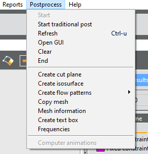
Start and Start traditional post open CompassFEM postprocess and GiD postprocess respectively.
End menu option closes postprocess and opens GiD preprocess again.
In order to toggle between pre and postprocess the following icon in the main toolbar must be pressed:
Only binary2 and ASCII result formats can be read in CompassFEM postprocess, so that if binary result format has been selected
when analysis was performed, a dialog box will appear to open Traditional postprocess.
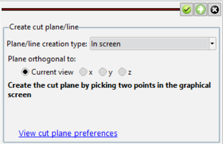
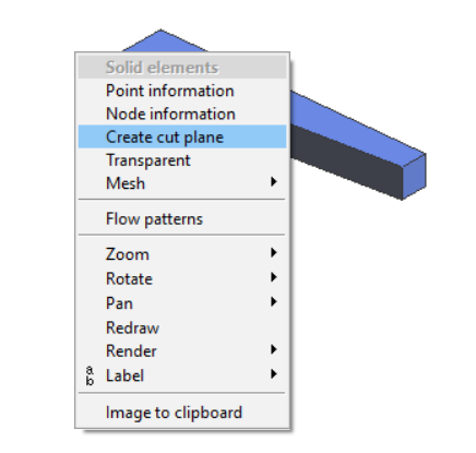
It is possible to define the cut plane by three ways:
In screen: picking two points in the screen a line will be created. The plane will contain this line. If this option is used, It must be chosen to use global axis as a normal vector to the cutting plane, or chosen the cutting plane is orthogonal to the current view.
Three points: the cut plane will be defined by three points.
Two points: the cut plane will contain the two defined points and will be orthogonal to current view.
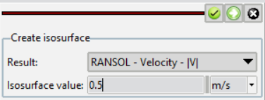
This option draws a surface or a line passing through all the points which have the same selected result’s value inside a volume mesh, or surface mesh. For doing it, a result must be chosen and a value must be indicated to create a isosurface.
Fig. 1.160 Isosurface panel. It is necessary to chose a result of the list and enter a value within the range of the result values.
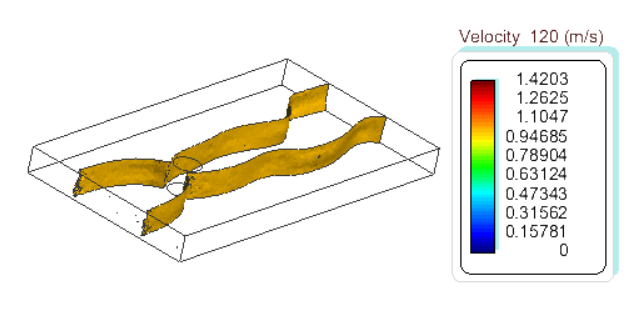
Fig. 1.161 Example of isosurface. Velocity of 1 m/s.
Postprocess allows to create flow patterns when there are fluid results. At least, it is necessary a fluid velocity result, but there can be fluid density result too.
There are three types of flow pattern that can be created. Following, these three types are described.
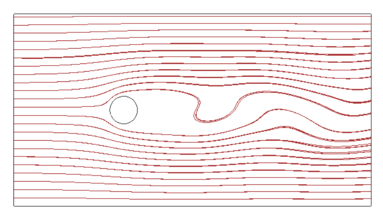
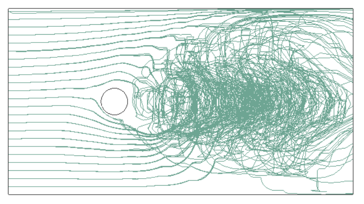
Streamlines are a family of curves that are instantaneous tangent to the velocity vector of the flow. These show the direction a fluid element will travel in at any point in time.
Pathlines are the trajectories that individual fluid particles follow. These can be thought of as a “recording” of the path a fluid element in the flow takes over a certain period. The direction the path takes will be determined by the streamlines of the fluid at each moment in time.
Fig. 1.164 Front view of particle tracking calculated with parameters shown above.
1.7.2.6.2. Creation and management of flow patterns
It is possible to draw flow patterns in two ways:
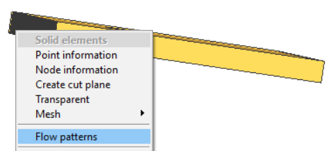
Selecting a mesh with the right button of the mouse and flow pattern option of contextual menu. The selected mesh must be the fluid domain or be related to the fluid domain (for example the inlet). If the chosen mesh is the fluid domain and it is plane, it must be in the Z plane.
Fig. 1.165 Contextual menu to create flow pattern.
Selecting the menu option. This menu option allows to choose the type of flow pattern, streamline, pathline or particle tracking.
A pane placed in the postprocess data tree allows to configure the flow pattern:
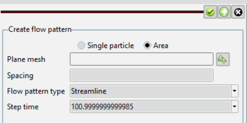
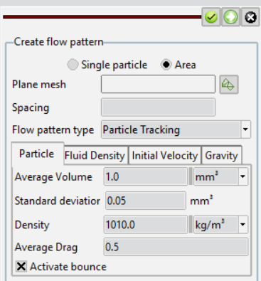
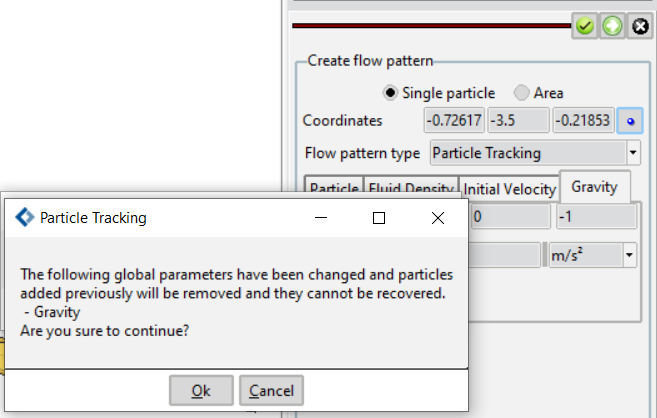
First of all it is necessary to select the scope of the flow pattern to create, Single particle or Area.
Single particle: a flow pattern of a particle will be drawn. If the flow pattern tool is selected by the contextual menu, the initial position of the particle will be the point where the mesh was selected. The initial coordinates are shown in the frame when this option is selected and it can be changed using the button at the right of the coordinates. The coordinates units are the same of the mesh ones. On the other hand, if the flow pattern tool is selected by the menu, the particle coordinates must be selected using the button.
Area: this option allows to create an area filled of particles. For using this option, a plane mesh must be selected (for example the inlet or a cut mesh). If flow pattern tool is selected using the contextual menu, the selected mesh will be used for creating the filled area of particles. If the menu is used, a mesh must be selected using the button at the right of the Plane mesh name. A boundary square around the mesh is calculated and it is filled of particles. The spacing between particles must be defined in the frame. The unit of the spacing is the same of the mesh one.
The next selector allows to choose the type of flow pattern to create. Although a type of flow pattern was selected using the menu, it is possible to change the type of flow pattern using this selector.
According to the type of flow pattern different options are available:
Streamline: a step time must be chosen among all steps calculated by the program.
Fig. 1.166 Streamline panel. It is necessary to choose a step value to create streamlines of this step.
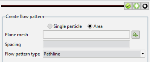
Pathline: there are not more options.
Fig. 1.167 Pathline panel. It is necessary to choose a step value to create streamlines of this step.
Particle Tracking: there are four groups of parameters:
Particle parameters: if Single particle option is selected, the particle parameters will be:
Volume
Density
Drag coefficient
Area parameters: if Area option is selected, the particle parameters will be:
Volume average of the particles
Standard deviation
Density
Drag coefficient average
The volume of each particle will be a random number from a Gauss distribution, and its drag coefficient will be calculated according its volume and the drag coefficient average.
Bounce: If this option is selected, particles will bounce off the mesh limit.
Fluid density:
Use density result: if there is a fluid density result selected in preferences (see Annex II: About the postprocess results file) Use density result can be selected or not. If not, Use density result cannot be selected. If it is unselected, a fluid density value must be defined. These values will be used for all particle tracking, thus it is strongly recommended to define these values for the first flow pattern and not to change them during all session.
Initial Velocity:
Use fluid velocity: if this option is selected the initial velocity of the particles will be the fluid velocity in their initial positions. If not, initial velocity of particles has to be defined by the user. These values will be used for all particle tracking therefore it is strongly recommended to defined these values for the first flow pattern and not to change them during all session.
Gravity: It is necessary to define gravity to calculate particle tracking. If this value is changed, then all particle tracking defined previously are removed.
Fig. 1.169 Gravity for particle tracking panel. If this value is changed, then all particle tracking defined previously are removed.
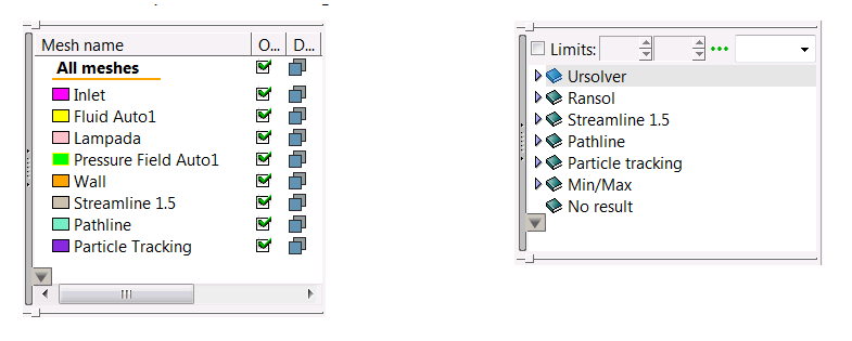
When all parameters are configured, the flow pattern is created. New point meshes are created for pathlines and particle tracking and for each step of streamline selected. Moreover, new results of displacement and velocity are created using the same classification.
Fig. 1.170 Meshes and results panels with meshes and results of created flow patterns.
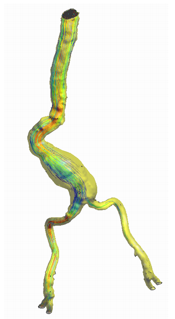
Fig. 1.171 Example of pathlines in a Abdominal Aortic Aneurysms
There are some preferences related to flow patterns in Preferences selector.
Please, see Preferences data tree manual for more information about the flow patterns preferences on the panel.
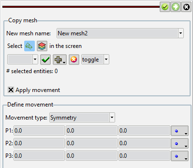
Copy mesh allows to copy a mesh, a group of meshes or a set of elements of a mesh
and apply a movement or symmetry to copied elements. The new meshes inherit the
results of the original meshes. This command is very useful when the model used for
calculating the results is a half or a fourth of the real model, and it is necessary
to show the results of the complete model. For example, the following model is
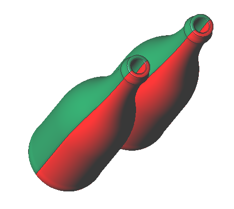
calculated using the half of the real model. Therefore, both meshes are copied and a symmetry
movement is applied. Below, the imported meshes from preprocessor (green) and the copied meshes (red).
Fig. 1.172 Example of copy mesh. The green ones are the original meshes and th red ones are the copied meshes.
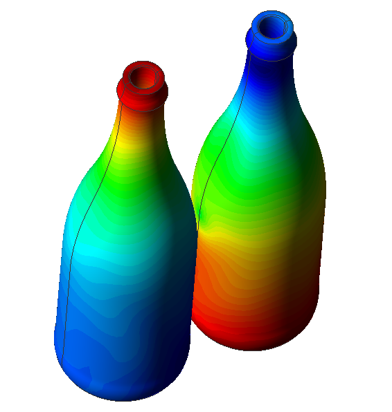
If a result is shown, it can see how the new meshes have inherited the results.
Fig. 1.173 Example of copy mesh with results. The new meshes inherit the results of the original meshes.
A mesh, several selected meshes or a set of elements of a mesh can be copied,
and it is possible to apply a linear movement or a symmetry.
Fig. 1.174 Copy mesh panel. It is possible to copy a mesh, a group of meshes or a set of elements of a mesh,
and apply a geometry transformation (movement or symmetry)
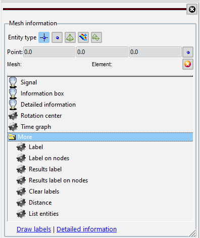
This command shows information of the following entities:
Point
Node
Element
Minimum and maximum result
Mesh
Fig. 1.176 Mesh information panel. It allows to get information about points, nodes, elements, etc….
Depending on the selected item, the panel has different options.
If the selected entity type is Point, Node, Element or Minimum and maximum result,
the most important information options are:
Signal: it is useful to find an entity in the screen.
Information box: an information box is shown with information of the entity as its
position or its result value (if a result had been selected before using this option).
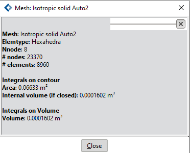
Detailed information: more information of the selected entity can be show with this option,
for example, the area or the volume of a mesh.
Fig. 1.177 Detailed information of a mesh. It is possible to know detailed information of
Point, Node, Element or Minimum and maximum result
Rotation center:
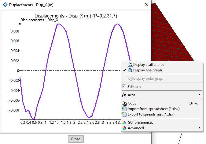
Time graph: if the performed analysis is dynamic or nonlinear, this option creates a graph with the selected result
information evolution in a point, node, element or the minimum and maximum result.
Fig. 1.178 Time graph of the selected result at a point and its contextual menu.
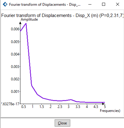
Contextual menu of Time graph allows to modify physical appearance of the graph, export and import. Advanced menu has several options and one of them allows to calculate Fourier transform of the time graph.
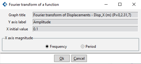
When Fourier transform graph is selected, a dialog window allows configuring its appearance.
Fig. 1.179 Fourier graph dialog. it allows to configure the graph.
Fourier transform will calculate from X initial value to first change of X increment, since it is possible to calculate Fourier transform if X increment is constant.
Fig. 1.180 When Fourier graph dialog is closed, a new graph is created with the Fourier transform of the original graph.
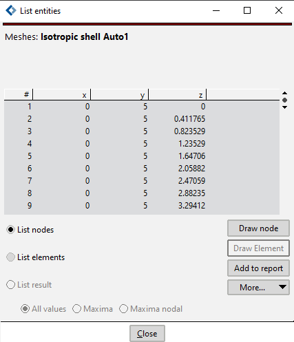
If the entity type is a Mesh, the most important information options are:
List entities: it allows to create lists of nodes (coordinates of all nodes), elements, or result value of all nodes.
It is necessary to select a result previously to show the result value of nodes or elements.
It is also possible to export the shown list to file.
Fig. 1.181 List entities window. It allows to create lists of nodes (coordinates of all nodes), elements, or result value of all nodes.
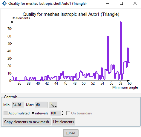
Mesh quality: it shows the quality of a selected mesh, for example the minium and maximum angle.
This option is not available por linear and hexahedra meshes.
Fig. 1.182 Mesh quality window. It shows the minimum and maximum angle and a graph of element angles.
This option is not available por linear and hexahedra meshes.
Hide elements: it allows to hide a selected group of elements. When this option is closed, then the hiden elements are shown another time.
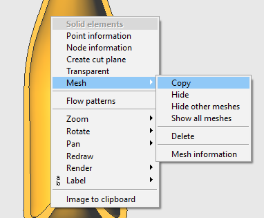
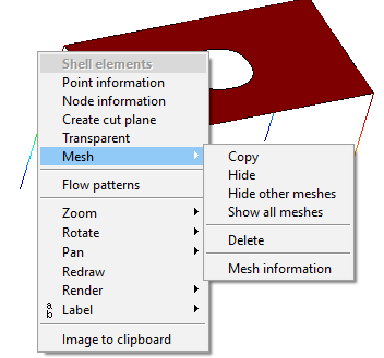
If an element is selected with the right button of the mouse, contextual menu will have several options for knowing mesh information.
Point information: it gives an information box about mesh entities and results when pressing on a point (data about the point and the result over it).
Moreover, more detailed information can be shown when clicking on the box, also data on nodes and Gauss points,
integrations over sets (both in global and local axes), local axes drawing, etc.
For surfaces, local axes will have z’ axe as normal. For lines, x’ axe will be tangent to line. For line cuts, z’ axe will also be normal to surface.
Node information: it gives information about the coordinates of the selected node.
Contextual menu >> Mesh >> Mesh information: it opens the Mesh information panel with the mesh options.
Fig. 1.183 Contextual menu allows to select Point information, Node information and Mesh information.
A text box is shown at the bottom of the screen with the selected combination loadcase, result and, if it is possible the time step or load step.
Fig. 1.184 Text box with the selected combination loadcase, result and, if it is possible the time step or load step. It is shown at the bottom of the screen.
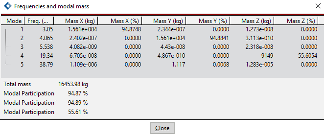
This options is only available when a modal analysis has been opened in Postprocess.
It opens a dialog box with frequencies and modal mass participation of calculated frequencies.
Please, see Ramseries Dynamic Conditions manual to know how configure a modal analysis.
Fig. 1.185 Frequencies and modal mass window. It is only available in modal analysis.
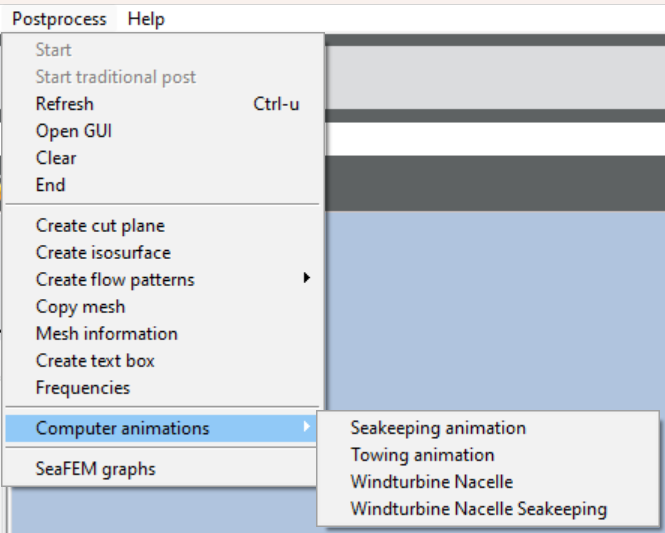
Once Postprocess is opened with a results file loaded, some animation templates are available in the Postprocess >> Computer animations menu.
Fig. 1.186 Postprocess menu with the available animations.
In this menu there are as many animations available as there are xml files in the folder folder_distribution/problemtypes/compassfem.gid/animations
It is important to note that the animations folder (problemtypes/compassfem.gid/animations)
of the installation directory offers various default template files in XML format
which are provided to be used for creating new animations automatically.
Furthermore, it is possible to add new template files into the animations folder of the installation directory for designing special animations in other particular models.
Nowadays, the following animations are available:
Seakeeping animation
Towing animation
Windturbine nacelle
Windturbine nacelle seakeeping
If the user opens the problemtypes/compassfem.gid/animations folder he will notice that there are xml files that do not appear in the Postprocess >> Computer animations menu.
Each of the files contains the following text:
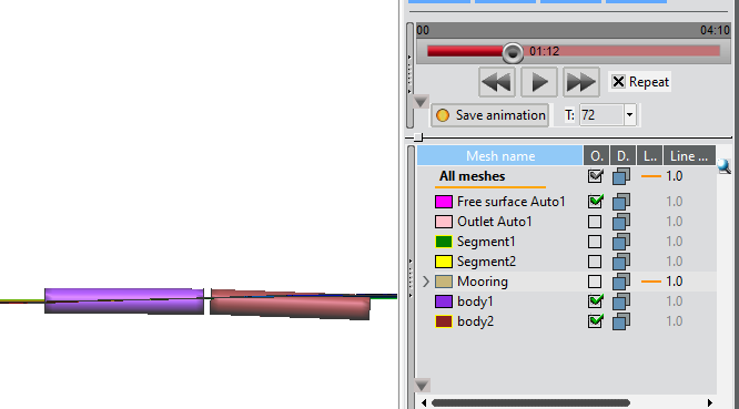
It is possible to perform animations with multiple bodies (100 or 200 or more).
To perform this animation, it is necessary to open a model calculated by SeaFEM with as many body meshes and body results as bodies must be moved
in the animations.
Body meshes files must be named according this pattern BodyN.msh where N is the number of the body.
Similarly, body movement results files must be named according this pattern BodyMovements_animations_N.res where N is also the number of the body.
However, the first body movement results file must be named BodyMovements_animations.res.
All these files must be stored in the SeaFEM analysis folder. When Postprocess >> Computer animations >> Seakeeping animation is selected,
All bodies meshes and movement results are read and animation is created.
Fig. 1.187 Example of multiple bodies animation.
If Play button is pressed, bodies are moved.
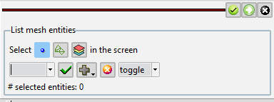
This command is available for structural models. It calculates total reactions in a model. When this menu option is selected, the following window is opened:
Fig. 1.188 This panel allows to select nodes, elements or meshes. In this context, this selection will be used to compose reactions.
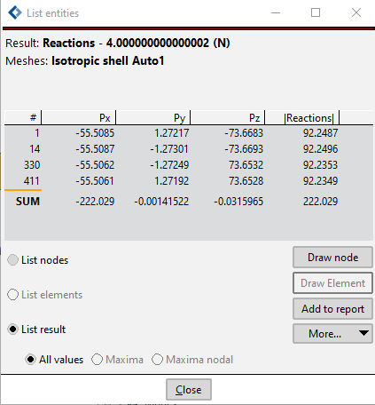
When List result is selected, then all reactions and their sum is shown:
Fig. 1.189 ‘List entities’ window shows nodes with reactions, and their sum.
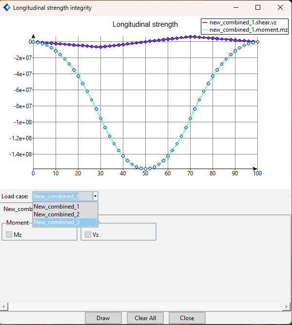
This command is available for structural models with hull girder results.
These results are calculated when they are selected in the Tdyn Data tree (General data > Results > Hull girder results> Calculate hull girder results).
When this menu option is selected, the following window is opened:
Fig. 1.190 ‘Longitudinal strength integrity’ window. It is possible to select multiple results of different combined loadcases.