The CompassFEM Postprocess provides four panels on the right of th GUI.
They allow to perform animations, change mesh display properties as colour or transparency,
select results and how to show them, and preferences.
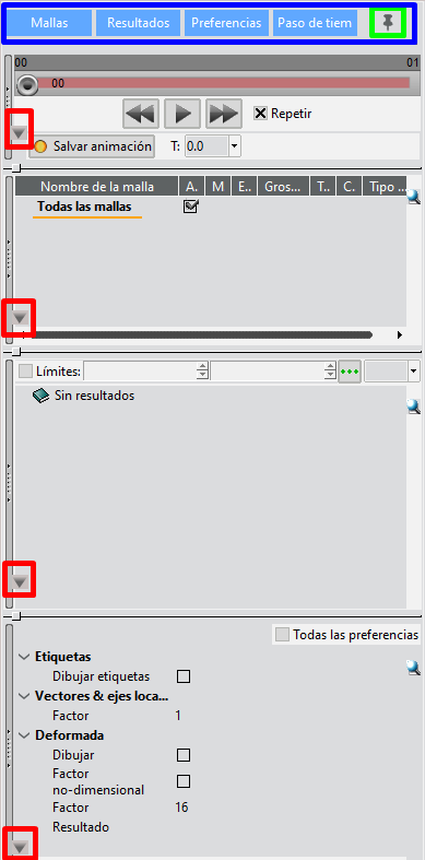
These panels can be shown, hidden or minimized using the buttons highlighted in the following image.
Fig. 1.193 The four panels provided by Postprocess can be shown, hidden or minimized using the buttons highlighted.
The four buttons highlighted with the blue circle can show and hide the panels and th buttons highlighted
with the red circle can minimize and maximize them. Moreover, the button highlighted with a green circle
allows to dock and undock the four panels to the GUI.
It is possible to animate dynamic simulations and static analysis if meshes have been deformed using a vector result.
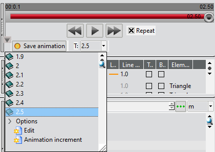
If a dynamic analysis is loaded a combo box allows to select a step of the selected result.
Fig. 1.194 The combo box shows the steps of the selected result and allows to choose one of them.
For example, the shown result of this simulation contains 25 steps from 0.1 to 2.5 s.
This combo box also allows to view Animation preferences
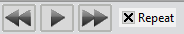
The Animation panel provides controls similar to a video player.
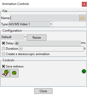
Moreover, it is possible to save the animation in a video file using Save animation.
Fig. 1.195 This panel allows to export the animation to AVI, MPEG or other video formats.
The procedure recommended to export to standard video format is explained below:
Define properties as name, type, delay, etc… Save redraws must be set.
Click button to start to save the animation.
Click button to start animation.
Click button to finish and close animation file.
The following explains how to make an animation of a static simulation.
1. Use Deformed preferences to select a vector result to deform meshes.
Configure other deformed parameters if it is necessary, and activate Draw in the Deformed preferences.
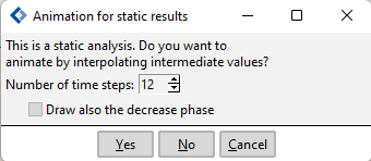
When the red slide bar of the Animation panel is clicked, then a dialog win is opened to define interpolated steps.
Fig. 1.196 Dialog window to define how to create interpolate steps in static results.
It is possible to define how many steps to create and if the decrease phase is drawn too.
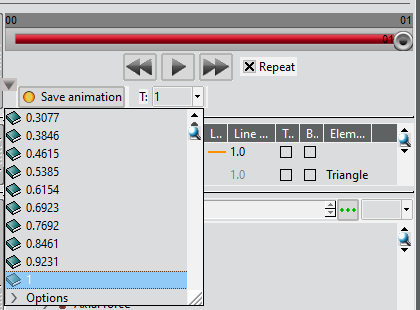
Now, interpolated steps have been created and it is possible to animate simulation as a dynamic analysis.
Fig. 1.197 Interpolated steps created in a static result when deformed configuration is activated.
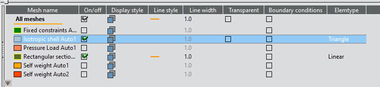
This panel shows all meshes contained in the model and allows to manage their visualization.
Fig. 1.198 Meshes selector. In structure models, only material meshes are shown when the model is read,
only fluid meshes are shown in CFDs or heat transference analysis.
Using Meshes selector any mesh can be shown or hidden.
The available display properties are as follows:
On/Off: mesh visualization.
Display style: Change the visualization style between the following options available:
Render
Render with border
Render and mesh
Mesh
Borders
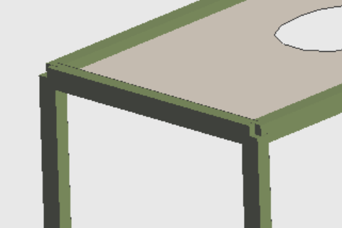
Line style: it is possible to draw shells and beams with real section.
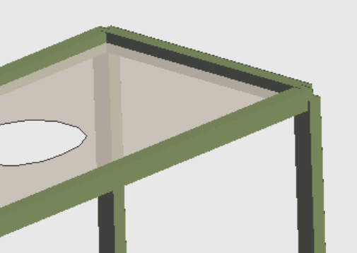
Fig. 1.199 Shell and linear meshes drawn with real section.
Transparent: manage the mesh surface transparency.
Fig. 1.200 The mesh surface can be drawn transparent or opaque.
Boundary conditions: it draws the selected mesh as boundary conditions. For example, in the next figure, Fixed constraints Auto1 mesh is drawn as Boundary conditions.
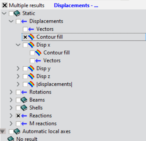
From this window it is possible to draw all calculated results using different type of visualizations (Vectors or Contour Fill).
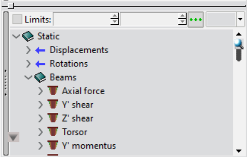
Fig. 1.202 Results panel allows to select one o several results to be drawn.
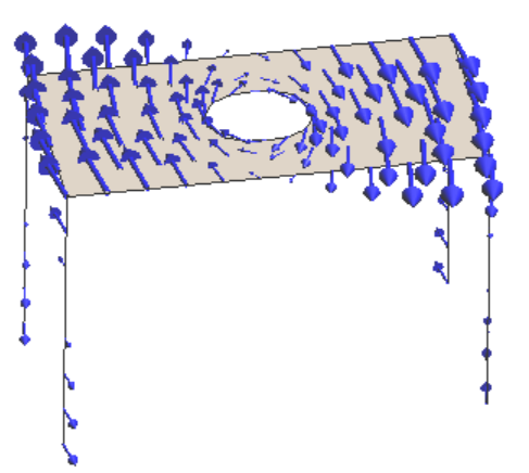
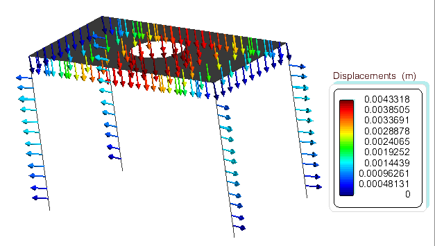
In the case of Vectors, then once a result is chosen, the program will display its nodal vectors.
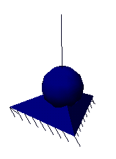
Fig. 1.203 Example of result drawn using vectors.
Vectors & Local axes preferences allows to define some visualization properties of vectors.
Contour Fill allows the visualization of colored zones,
in which a variable or a component changes between two predefined values.
Fig. 1.204 Contour fill result. Result values are drawn using a colours map.
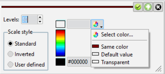
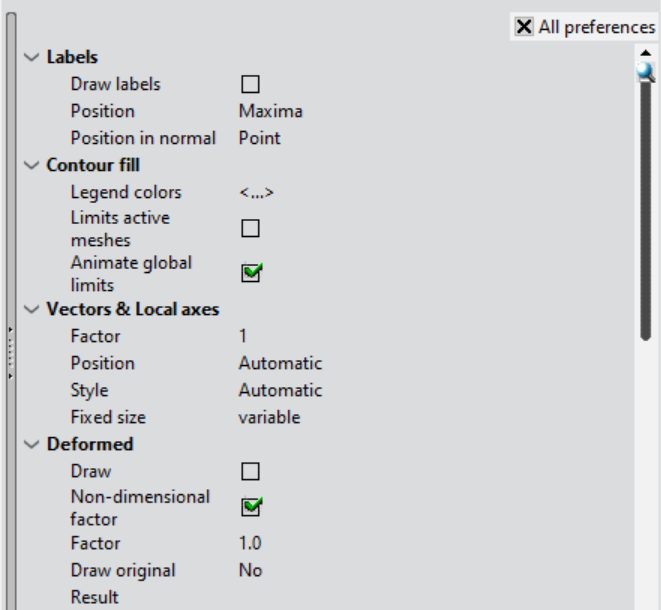
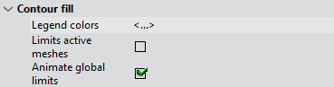
The Legend colors can be configured in Contour fill preferences
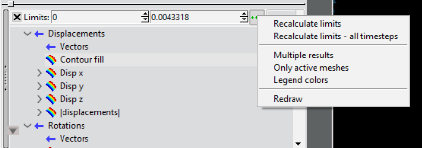
It is possible to fix maximum and minimum limits for the color scale,
which can also be calculated automatically for the active meshes or for all the meshes.
The following figure shows controls to define limits for the color scale and the contextual menu that allows to recalculate the limits.
Fig. 1.205 Values limits of contour fill result can be managed using the controls on the top of the Results selector.
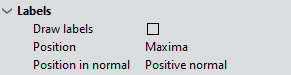
If Draw labels is activated, labels are drawn on the model depending on the context and the value of the preferences.
If a result is selected, then the labels show the result value to the node.
If Position is All, there are a label for each node,
but if Position is Maxima then only where the result is the maximum.
If no result is selected, then the labels show the number of node.
In this case, there are labels for each node although Position is
Maximum.
Fig. 1.209 Preferences for labels. It is possible to draw labels on the model depending on the context and the value of the preferences.
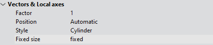
This preferences allows to configure Vector and Local axes results.
It is possible to modify the size factor,
the position in all nodes or only some of them (Automatic),
the arrow style (Line or Cylinder) and if size is fixed or variable.
Fig. 1.211 Preferences for Vector and Local axes results.
Fig. 1.212 If Vector size is fixed, then all vectors are the same size and their color is different
based on the legend colors.
Meshes can be deformed according to a vector result and a factor.
When doing this, all results are drawn on the deformed meshes.
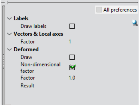
Draw: if it is activated, the deformed configuration is drawn.
Adimensional factor: if it is activated, then the deformed configuration size is not real and the optimum visualization is used.
Factor: factor which multiplies the deformed configuration. If factor = 1 and adimensional factor option is not checked, the visualization is real.
Draw original: it allows to draw the original configuration (without any deformation)
and to choose the visualization style (render, render with border, render and mesh, mesh or borders).
Result: a vector result must be chosen. This result is used to show the deformed configuration.
Please see Animation control to know how to animate the deformed configuration.
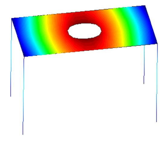
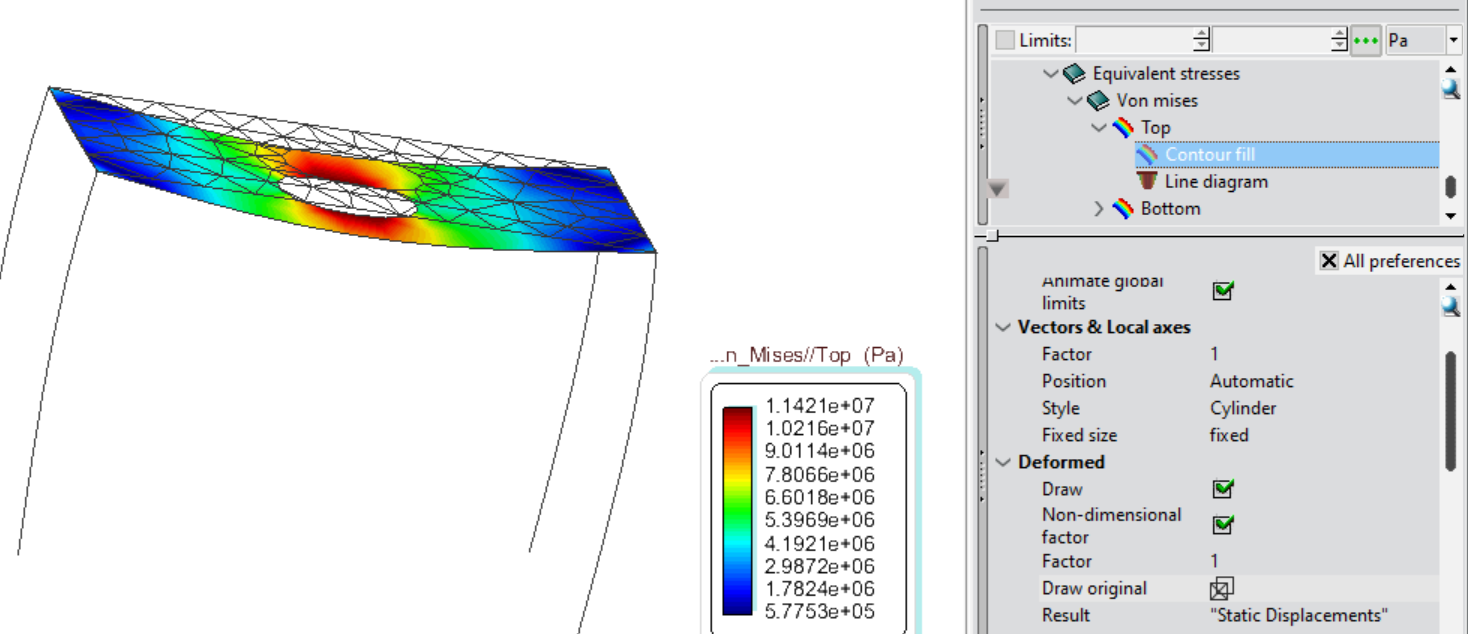
Fig. 1.213 Example of deformed configuration. Static displacements result is selected to define deformed configuration and Von mises on the top surface is
selected to draw on the model. Moreover, Non-dimensional factor is activated to allow the deformed configuration to be visible,
and original configuration is drawn in the Mesh style.
Auto extend cuts: when creating a cut over one surface, the cut line extends as much as possible.
If cut plane is created using menu option, the cut line is extended regardless of this preference.
However, if cut plane is create using the contextual menu, then the cut line is extended depending on this preference.
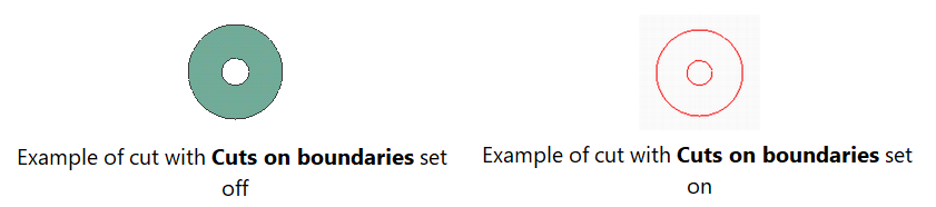
Cuts on boundaries: if selected, the cuts on volumes will be lines on the boundary of the volume.
Auto transparent: when a cut over a surface or volume is created, then the new mesh is set automatically to transparent.
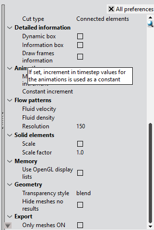
Cut type: this option defines the way that a plane cuts the set of active meshes:
Connected elements: only are considered the element under the cursor and elements connected to it, without crossing aristes.
Mesh: only are considered the elements that belongs to the mesh under the cursor.
All: the created plane cuts all active meshes.
Please, see Create cut plane to know more information about cut plane creation.
These are the preferences that can be configured for flow patterns:
Fluid velocity: this is the most important preference related to flow patterns.
It makes possible to choose a fluid velocity result necessary for creating flow patterns.
Postprocess tries to find it, but if it is not possible, then user will have to do it.
If there is not any fluid velocity result chosen, flow patterns will not be able to be created.
Fluid density: it makes possible to choose a fluid density result.
If there is not any fluid density result chosen, a fix density value must be defined in the particle tracking window.
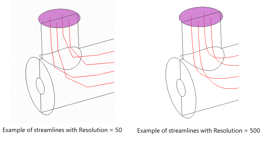
Resolution: It is the number of points to be drawn for all flow patterns.
Between each pair of points, a straight line will be drawn.
Therefore the higher resolution, the smother will be flow patterns.
When it is changed, all flow patterns will be recalculated and redrawn using the new value.
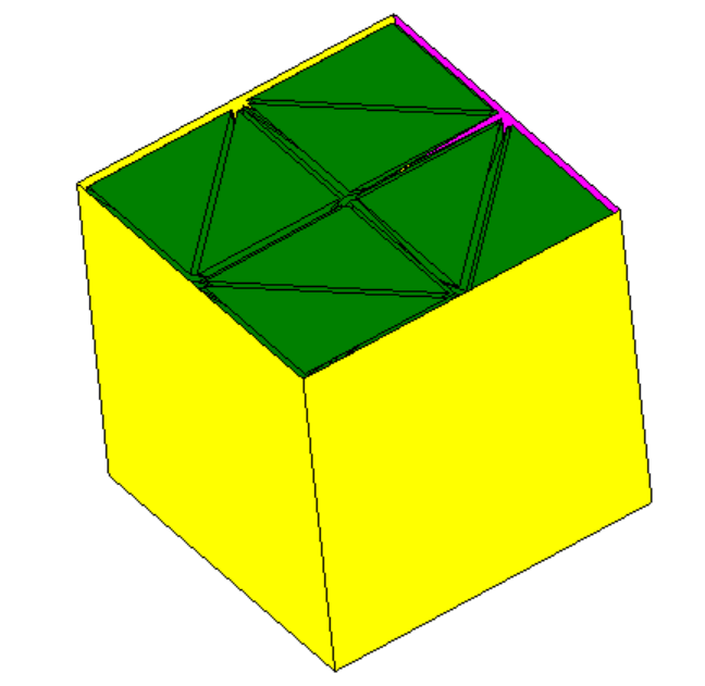
Draw tetrahedra and hexahedra with reduced size, in order to separate them from neighbours.
If Scale factor is less than one, then the elements are reduced.
Fig. 1.214 Example of solid scale factor. In this case, factor = 0.9