Fluid dynamics and Multiphysics data refers to all the information
required for performing the analysis and it does not concern
any particular module. Fluid dynamics and Multiphysics data also differs
from the previous definitions of conditions and materials
properties, which are assigned to different entities. Some
examples of general Fluid dynamics and Multiphysics data are the type of
solution algorithm used by the solver, the value of the time
step, convergence conditions and so on.
This group of data refers to the selection of problems to be
solved with Fluid Dynamics and Multiphysics.
Solve fluid:
Select this option if you are going to solve any fluid problem. If this option is not selected, any defined fluid domain will be ignored in the solution of the problem. Several options exist for Solve fluid:
Solve Fluid Flow : Select this option if you are going to solve fluid flow (RANSE) problem. This option will only be available in Fluid Flow module.
Solve heat transfer : Select this option to solve a heat transfer problem in a fluid. If this option is not selected, the temperature problem in fluid domains will be ignored in the solution process. This option will only be available in Heat Transfer module.
Solve Species advection: Select this option to solve a species advection problem in fluid. If this option is not selected, the species advection problem in fluid domains will be ignored in the solution. This option will only be available in Species Advection module.
Solve PDEs problems: Select this option to solve any user defined PDE (phi variables) problem in fluid. If this option is not selected, the user defined PDE’s problem in fluid domains will be ignored in the solution. This option will only be available in PDE’s solver module.
Solve free surface (ODDLS): Select this option to solve free surface problems in fluid based on ODD level set. This option will only be available in ODDLS module.
Solve free surface (Transpiration): Select this option to solve a transpiration free surface problem in fluid. If this option is not selected, the transpiration free surface problem in fluid domains will be ignored in the solution. This option is only available in Transpiration module of 3D analysis.
Solve mesh deformation: Select this option to apply mesh deformation algorithms and apply Arbitrary Lagrangian Eulerian (ALE) solvers in fluid. This option will only be available in Mesh Deformation module.
Solve comfort: Select this option to solve comfort problems in fluid domains. This option will only be available in Comfort module.
Solve solid :
Select this option if you are going to solve any solid problem. If this option is not selected, any defined solid domain will be ignored in the solution of the problem. Several options exist for Solve solid:
Solve Solid Flow: Select this option if you are going to solve fluid flow problem in a solid (flow in porous media). This option will only be available in Flow in Solids module.
Solve heat transfer: Select this option to solve a heat transfer problem in a solid. If this option is not selected, the temperature problem in solid domains will be ignored in the solution process. This option will only be available in Heat Transfer module.
Solve species advection: Select this option to solve a species advection problem in solid. If this option is not selected, the species advection problem in solid domains will be ignored in the solution. This option will only be available in Species Advection module.
Solve PDEs Problems: Select this option to solve any user defined PDE (phi variables) problem in solid. If this option is not selected, the user defined PDE’s problem in solid domains will be ignored in the solution. This option will only be available in PDE’s solver module.
Number of Steps:
Number of steps of the simulation. Total physical time to be simulated will be Number of Steps x Time increment. Recommended values to achieve steady state is:
\[NumberOfSteps ≥ 1000·dt·V/Ld\]
where dt is the time increment and V, Ld the characteristic velocity and length.
Time Increment:
Time step of the simulation. Total physical time to be simulated will be Number of Steps x . The recommended value is:
\[dt=C·Ld/V\]
where dt is the time increment, V, Ld the characteristic velocity and length and 0.1 < C < 0.01.
In case a transient phenomenon of characteristic time or period (T) is expected, then dt can be calculated as 1/10 to 1/100 of T of the problem is usually more appropriate.
Note
Remarks:
In any case, it is important to verify if the dt calculated with the above formulae is adequate for the mesh used. This can be done by evaluating a characteristic mesh time as: dtm = h/V,
where h is the characteristic mesh size (usually the smallest element size). It is recommended the dt used in the calculations to be between 2·dtm < dt < 20·dtm.
Time increment may also be defined by a global function (see Function Syntax section for further information). Units of the time step of the simulation are given in the menu next to this field.
Mas Iterations: Maximum number of iterations of the non-linear algorithm for solution of the problem. Recommended values come from 3 to 10, depending on the value of the convergence norms (see Modules Data section).
Note
Remarks:
In some cases the algorithm may not converge in the initial time-steps, due to the start up process, resulting in the appearing of a warning message More than…number…iterations may be necessary. If only the steady state is of interest, this message may be simply ignored, otherwise Max Iterations value should be increased.
Initial Steps: During first Initial Steps some controls are carried out in the algorithm in order to stabilise the problem during the start up process. It is strongly recommended to define Initial Steps about 10% of the Number of Steps in problems with free surface transpiration.
Start Up Control: if activated, during first Initial Steps the start up process is smoothed. This can be done by creating a adequate acceleration in the flow (Speed), by smoothly increasing the time increment (Time) or Both.
Restart: if On, the restart file is used to define the initial data. The Restart file taken will be ‘ProblemName.flavia.rst’. This file is automatically written with the rest of the results. To restart a case, the Number of Steps must be increased in the number of new steps to be run.
Note
Remarks:
Note that the Number of Steps must be set to a number greater than the last step reached in the previous calculation. For example, if one should want to restart and perform a calculation of 100 steps, and the previous calc. reached 600, the Num. of Steps should be set to 700.
Processor unit: it allows to choose between CPU and CPU+GPU processor options. If CPU mode is selected the entire calculation is performed in the Computer Processor Unit. On the contrary, if CPU+GPU mode is selected the numerical solver runs on the Graphical Processor Unit if this type of device is available in the computer being used. CPU+GPU mode tries to benefit from the increasing computational power of modern GPU devices in order to increase solver performance.
Multiprocessor mode: it allows to select the parallel execution mode. By default, Parallel mode is used so that the program automatically makes use of the maximum available number of logical CPU cores. If Sequential mode is used instead, the solver runs sequentially so that the program executes in a single logical processor. If the User Defined option is chosen, the user is allowed to select the actual number of logical CPU cores to be used during the calculation.
Number of CPU’s: Number of CPU’s is the number of processors to be used on a parallel computation. It must be less or equal to the maximum number of available processors in the current computer. In multi-core CPU machines, Number of CPU’s actually refers to the total number of independent cores.
Use Hypre Solvers: it allows to activate/deactivate the use of Hypre’ solvers. Hypre is a software library of high performance preconditioners and solvers for the solution of large, sparse linear systems of equations on parallel computers developed by the LLNL (Hypre’s site). It has been introduced in Tdyn to provide the capability of running parallel jobs using the message passing interface (MPI) paradigm.
MPI: it allows to activate/deactivate the message passing interface (MPI) parallel mode. It is only available when the Hypre Solvers option is active. Depending on the actual architecture and/or operating system of the computer, MPI execution may also require the installation of third party software responsible for the management of the parallel processes execution (see additional information on the CompassIS webpage).
Number of MPI nodes: when using the MPI parallel execution mode, this entry allows the user to specify the number of calculation nodes to be used for parallel execution. Based on this information, Tdyn will automatically perform the required domain decomposition before running the calculation.
Steady State solver: if On, it starts the calculation procedure for an automatic search of the steady state.
Output Step : each Output Step time steps the results will be written to disk.
Note
Remarks:
This value will control the size of the results file.
Output Start: the results will be written each Output Step time steps after Output Start steps.
Note
Remarks:
This value will control the size of the results file.
Results File: type of the results file (Binary, Binary2, ASCII or EnSightGold). Binary2 must be used to visualize results with CompassFEM postprocess. Binary can only be read by the Traditional postprocess. However, the Traditional postprocess can read also Binary2 results, so it is not recommended to use Binary format.
Fluid Flow: options available with Fluid Flow module selected.
Write Initial Data : mark to write in the results file the initial data of the problem.
Write Velocity : mark to write velocity field in the results file.
Write Velocity Stress Tensor: mark to write velocity stress tensor field in the results file.
Write Pressure : mark to write pressure field in the results file.
Write Pressure Gradient: mark to write pressure field in the results file.
Write Total Pressure: mark to write total pressure field in the results file (including hydrostatic component).
Write Density : mark to write fluid density field in the results file.
Write Viscosity: mark to write viscosity field in the results file.
Write Wall Law Traction: mark to write wall stress given by the Law of the Wall (if exits) in the results file.
Write Tau Parameter: mark to write tau parameter (local Courant number) field in the results file.
Write Eddy Viscosity: mark to write eddy viscosity field in the results file.
Write Eddy Kinetic Energy: mark to write eddy kinetic energy field in the results file.
Write Epsilon: mark to write epsilon (turbulence variable) field in the results file.
Write Omega: mark to write omega (turbulence variable) field in the results file.
Write K Tau: mark to write kτ variable (of K_KT turbulence model) field in the results file.
Heat Transfer: options available with Heat Transfer module selected.
Write Temperature: mark to write temperature field in the results file.
Write Temperature Gradient: mark to write temperature gradient field in the results file.
Write Heat Flux: mark to write heat flux through the boundaries.
Write Solid Density: mark to write solid density field in the results file.
Species Advection: options available with Species Advection module selected.
Write Species Concentration: mark to write species concentration field in the results file.
PDE’s solver: options available with PDE’s solver module selected.
Write Phi Variable: mark to write phi variables field in the results file.
Mesh Deformation: options available with Mesh Deformation module selected.
Write Mesh Deformation: mark to write mesh deformation in the results file.
Write ALE Velocity: also referred as Eulerian velocity. Mark to write the velocity given in the moving reference frame.
Free surface: options available with free surface (transpiration) module.
Write Wave Elevation: mark to write wave elevation field in the results file.
Write Wave Elevation Vector: mark to write wave elevation vector field in the results file.
Comfort module: options available with comfort module.
Write PMV: mark to write PMV index results (Predicted Mean Vote).
Write PPD: mark to write PPD index results (Predicted Percentage Dissatisfied).
User defined functions: options available to provide user defined results. Each custom results may be written as a function of already available problem variables.
Fluid Function #: Mark to write the function field (only evaluated in fluid domain) in the results file. The function field is written in IS units in the analysis group USERDEF. If this file is marked, two new field will be available.
Name: Name of the function. The corresponding field is identified with this name in the postprocessing part.
Function: Insert the fluid function to be evaluated and written. See Function Syntax section for further information.
Solid Function #: Mark to write the function field (only evaluated in solid domain) in the results file. The function field is written in IS units in the analysis group USERDEF. If this file is marked, two new field will be available.
Name: Name of the function. The corresponding field is identified with this name in the postprocessing part.
Function: Insert the fluid function to be evaluated and written. See Function Syntax section for further information.
1.2.2.1.4. Options available in Fluid Solver section
This group of data refers to all the information required to define the integration scheme and solver data of the problem/s to be analysed in the fluid domain.
Flow Solver Model: Flow solver model used in the fluid domain. Available options are Incompressible, PrCompressible (compressible algorithm using pressure as main variable) and DnCompressible (compressible algorithm using density as main variable).
Incompressible model is adequate for those problems where the compressibility effects are small, as happens in open flows with characteristic Mach number below 0.4. It can handle small compressibility effects using the SlightlyIncompressible fluid model algorithm. See Materials section for further information.
PrCompressible is a compressible using pressure as main variable. This model is suitable for most of the practical cases. However it can not handle shock waves.
DnCompressible model is the most suitable for those problems where compressible effects are quite relevant. It can even simulate shock waves.
Time Integration: Time integration scheme used in the solution process of the fluid problem:
Backward Euler: Implicit 1st order scheme.
Crank Nicolson : Implicit 2nd order scheme.
Solver NonSymmetric: Solver type used in the solution of the nonsymmetric linear systems of equations.
Tolerance: Tolerance used in the solution of the non-symmetric linear systems of equations (see Solver NonSymmetric). A value smaller than 1.0·10-6 is recommended.
Max. Iterations: Maximum number of iterations of the nonsymmetric linear systems of equations (see Solver NonSymmetric).
Preconditioner: Preconditioner used in the solution of the nonsymmetric linear systems of equations (see Solver NonSymmetric).
Note
Remarks:
In some cases using elements with high aspect ratio the diagonal preconditioner may work better than others.
Krilov sp. dimension: Dimension of internal direct solver used in GMRes solver (see Solver NonSymmetric). A value greater than 20 is recommended.
Solver Symmetric: Solver type used in the solution of the symmetric linear systems of equations.
Tolerance: Tolerance used in the solution of the symmetric linear systems of equations (see Solver Symmetric). A value smaller than 1.0·10-6 is recommended.
Max. Iterations: Maximum number of iterations of the symmetric linear systems of equations (see Solver Symmetric).
Preconditioner: Preconditioner used in the solution of the symmetric linear systems of equations (see Solver Symmetric).
Note
Remarks:
In some cases using elements with high aspect ratio the diagonal preconditioner may work better than others.
Krilov sp. dimension: Dimension of internal direct solver used in GMRes solver (see Solver Symmetric). A value greater than 20 is recommended.
Advection Norm: Euclidean convergence norm of the velocity, used for recalculating or not advective terms. A value smaller than 1.0·10-5 is recommended.
Steady State Norm: Euclidean norm used to detect the steady state. If each variable increment is smaller than this norm, the problem is stopped and results are written to the disk.
Increment Control: This option activates a control that limits the maximum admissible increment of the variables for every iteration. The limit is taken as ratio of the convergence norm of the variable. Select None to switch this control off.
1.2.2.1.5. Options available in Solid Solver section
This group of data refers to all the information required to define the integration scheme and solver data of the problem/s to be analysed in the solid domain.
Flow Solver Model: Flow solver model used in the fluid domain. Available options are Incompressible, PrCompressible (compressible algorithm using pressure as main variable) and DnCompressible (compressible algorithm using density as main variable).
Incompressible model is adequate for those problems where the compressibility effects are small, as happens in open flows with characteristic Mach number below 0.4. It can handle small compressibility effects using the SlightlyIncompressible fluid model algorithm. See Materials section for further information. See Materials section for further information.
PrCompressible is a compressible using pressure as main variable. This model is suitable for most of the practical cases. However it can not handle shock waves.
DnCompressible model is the most suitable for those problems where compressible effects are quite relevant. It can even simulate shock waves.
Time Integration: Time integration scheme used in the solution process of the solid problem:
Backward Euler: Implicit 1st order scheme.
Crank Nicolson : Implicit 2nd order scheme.
Solver Symmetric: Solver type used in the solution of the symmetric linear systems of equations.
Tolerance: Tolerance used in the solution of the symmetric linear systems of equations (see Solver Symmetric). A value smaller than 1.0·10-6 is recommended.
Max. Iterations: Maximum number of iterations of the symmetric linear systems of equations (see Solver Symmetric).
Preconditioner: Preconditioner used in the solution of the symmetric linear systems of equations (see Solver Symmetric).
Note
Remarks: In some cases using elements with high aspect ratio the diagonal preconditioner may work better than others.
Krilov sp. dimension: Dimension of internal direct solver used in GMRes solver (see Solver Symmetric). A value greater than 20 is recommended.
Steady State Norm: Norm used to detect the steady state. A value smaller than 1.0·10-5 is recommended.
Increment Control: This option activates a control that limits the maximum admissible increment of the variables for every iteration. The limit is taken as ratio of the convergence norm of the variable. Select None to switch this control off.
User Defined Integrals
Within this section of the data tree, the user can define fluid and solid volumetric integrals of any of the calculation variables.
This integrals will be calculated for each time step.
Tcl data
Use Tcl External Script: If the check-box is selected, the Tcl extension is activated. The entry may indicate a Tcl script to be
interpreted during execution. The Tcl script can define any of the standard program Tcl functions. See section Tcl Extension
for further information about Tcl extension.
Other data
Warn. Level: If None, warning messages are not shown during the calculation process. Other possibilities are Few, Some or All.
Multiple Runs & Additional Steps: This options allows the user to create a vector of factors, which will affect the velocity field each
additional run (which will run for # additional_steps). For example, if multiple_runs=[1.0 1.51.6] and additional_steps=100,
then, when the first run finishes, a new run will start, for 100 steps, with the velocity field multiplied by 1.5. Again, when it
finishes, the resulting vel. field will by multiplied by 1.6, and the calculation will run for another 100 steps.
Mesh Refinement Type: This option tells Tdyn to calculate some mesh correction parameters, while the analysis is running.
These corrections are written in a file (background mesh, ***.bgm), and the mesher will read this file, modifying the mesh assigned
sizes, in order to improve it.
Modules data refers to all the specific information needed to performance a particular Tdyn CFD+HT analysis.
See Introduction section for more information about Tdyn CFD+HT modules.
Tdyn CFD+HT Modules Data options can be set from Modules Data in the tree.
Use Total Pressure: Mark if you want to use total pressure
(including fluid-static term) as internal variable in the solution of
the fluid flow problem.
Note
Remarks:
In most of the cases the solution of the fluid problem
without fluid-static term is the most accurate one. The “Use
total pressure” option is hence deactivated by default since
the pressure calculation algorithm is usually more precise.
It is recommended to activate this option only when fluidstatic (or more usually hidrostatic) effects are expected to
have a significant effect in the problem under analysis. If
this option is selected, please check the correctness of the
pressure boundary conditions. You must ensure that such
conditions take into account the fluid-static pressure term.
Pressure reference location: Mark if you want to define the origin of the fluid-static pressure term.
Pressure Origin: Coordinates of the total pressure origin.
Xplane Symmetry in Fluid: Mark if you want to define symmetry planes in the fluid problem, perpendicular to OX axis.
Xplane Symmetry Position: Position of the symmetry planes in the fluid problem, perpendicular to OX axis, given in the units of the geometry.
Yplane Symmetry in Fluid: Mark if you want to define symmetry planes in the fluid problem, perpendicular to OY axis.
Yplane Symmetry Position: Position of the symmetry planes in the fluid problem, perpendicular to OY axis, given in the units of the geometry.
Zplane Symmetry in Fluid: Mark if you want to define symmetry planes in the fluid problem, perpendicular to OZ axis.
Zplane Symmetry Position: Position of the symmetry planes in the fluid problem, perpendicular to OZ axis, given in the units of the geometry.
Operating Pressure: this is the reference pressure for compressible solvers. It is always taken into account to evaluate compressibility effects. The user must introduce pressure boundary conditions in accordance to the operating pressure value introduced in this field. In this sense, if for instance the atmospheric pressure is the actual value of the operating pressure introduced in this field, then you can fix the outlet boundary condition equal to zero and the inlet pressure equal to the actual inlet overpressure. On the contrary, if you use a cero pressure value as the operating pressure, then you must fix the outlet pressure boundary condition equal to the atmospheric pressure, and the inlet boundary condition equal to the atmospheric pressure plus the corresponding overpressure. In fact, both cases will provide the correct density, but only using the second approach you will also obtain the actual absolute pressure and total force over bodies.
Velocity Advect Stabilisation: Order of the FIC advection stabilisation term in the Navier Stokes equations.
Three available options are Auto, 4th_Order and 2nd_Order.
Note
Remarks:
The 4th order term increases the accuracy of the
solution and is recommended in most of the cases.
However in some problems it may cause
instabilities.
Auto mode will automatically switch between 4th
and 2nd order scheme, depending on the
smoothness of the solution.
Velocity Control Level: Level of control of instabilities (0 means
Off). If instabilities are found in the velocity field when using the
2nd_Order Velocity Advect Stabilisation, first try to reduce Time
Increment, then to increase this value. Note that high values
may cause over-diffusive results.
TauCalcType: This indicates the method for calculating the
stabilisation parameter tau. This should not be changed from its
default value (geometrical), for most of the cases. Nevertheless,
analytical method gives good results in cases where boundary
layer mesh is involved.
StabTauV MinRatio: Minimum admissible ratio (τ/dt, being dt the
time increment) for the stabilisation parameter τ of the velocity
solver. It will be also used for temperature and advection of
species problems.
Note
Remarks:
Advection stabilisation term is proportional to the parameter τ. In most of the cases, the minimum
value of this parameter should not be fixed (i.e. τ/dt = 0.0), otherwise oscillations may appear.
Velocity Inner Iterations: Number of iterations of the inner
nonlinear fluid flow momentum eq. solver (performed every
external iteration).
Velocity Norm: Velocity Euclidean norm used to check convergence in the non-linear iteration loop.
Velocity Boundary type: AdvancedVBC implements specific treatment
of boundary conditions for momentum equation in those boundaries with transient velocity conditions.
Pressure Stabilisation: Scheme to be used in the stabilisation
of the Pressure solver of the Navier Stokes equations.
StabTauP min. ratio: Minimum admissible ratio (tau/dt) for the stabilization parameter
tau used in the pressure stabilization.
StabTauP max. ratio: Maximum admissible ratio (tau/dt) for the stabilization parameter
tau used in the pressure stabilization.
Pressure Inner Iterations: Number of iterations of the inner nonlinear
Navier Stokes pressure solver (performed every external iteration).
Pressure Norm: Pressure Euclidean norm used to check convergence in the non-linear iteration loop.
Pressure Boundary type: AdvancedPBC implements specific treatment of boundary conditions
for mass balance equation in those boundaries with transient velocity conditions.
Initialise Flow Field: If Potential_Flow is selected, then the initial velocity
and pressure field is taken from the adaptation of the solution of a potential flow problem,
trying to the imposed boundary conditions. The available options are None, Potential_Flow and Stokes_Flow.
Floatability by Density: This must be activated if the floatability forces existing in fluids,
due to changes in density, are to be simulated.
Turbulence Model: Select the turbulence model to be used in the solution of the fluid flow problem.
Laminar: Navier Stokes equations are solved (i.e. Reynolds stress tensor is neglected and therefore
only direct simulation of turbulence is done).
Mixing_Length: Basic turbulence model based in the Prandtl hypothesis,
where the turbulence length scale (L) is given in the EddyLen Field entry.
Smagorinsky: Basic large eddy simulation (LES) turbulence model.
The implementation includes an eddy viscosity damping in the boundary layer area.
See Turbulence Modelling section for further information.
Kinetic_Energy: Prandtl’s one equation (k) model for turbulent flows with integration to the wall,
where the turbulence length scale (L) is given in the EddyLen Field entry.
K_Energy_Two_Layers: Prandtl’s one equation (k) model for turbulent flows with integration to the wall,
where the turbulence length scale (L) is given in the EddyLen Field entry.
The implementation of this model includes an eddy viscosity damping in the boundary layer area.
K_E_High_Reynolds: Two-equation k-ε model for turbulent flows.
The model implemented is based on the standard formulation with some modifications to be used with different wall boundary conditions.
See Turbulence Modelling section for further information.
K_E_Two_Layers: Two-equation k-ε model for turbulent flows with integration to the wall.
This implementation uses the high-Re k-ε model only away from the wall in the fully turbulent region,
and the near-wall viscosity affected layer is resolved with a one-equation model involving a length-scale prescription.
See Turbulence Modelling section for further information.
K_E_Lam_Bremhorst: Two-equation k-ε model for turbulent flows with integration to the wall.
The model implemented is based on the description done by Lam-Bremhorst with some modifications to be used with different wall boundary conditions.
See Turbulence Modelling section for further information.
K_E_Launder_Sharma: Two-equation k-ε model for turbulent flows with integration to the wall.
The model implemented is based on the description done by Launder and Sharma with some modifications to be used with different wall boundary conditions.
See Turbulence Modelling section for further information.
K_Omega: Two equation k-ω model for turbulent flows with integration to the wall.
The model implemented is based on the description done by Wilcox with some modifications to be used with different wall boundary conditions.
See Turbulence Modelling section for further information.
K_Omega_SST: Two-equation model for turbulent flows with integration to the wall, expressed in terms of a k-ω model formulation.
The k-ω SST shear-stress-transport model combines several desirable elements of standard k-ε and k-ω models.
See Turbulence Modelling section for further information.
K_KT: Two-equation k-kτ model for turbulent flows with integration to the wall.
The model implemented is based on the description done by Wilcox with some modifications to be used with different wall boundary conditions.
See Turbulence Modelling section for further information.
Spalart_Allmaras: One equation model for turbulent flows with integration to the wall.
See Turbulence Modelling section for further information.
ILES: Implicit LES model based on Finite Increment Calculus formulation.
Note
Remarks:
For further information about the turbulence models and how to solve turbulence flows,
please consult the Tdyn’s Turbulence Handbook.
Turbulence Advect Stabilisation: Order of the FIC advection stabilisation term in the turbulence equations.
Three available options are Auto, 4th_Order and 2nd_Order.
Note
Remarks:
The 4th order term increases the accuracy of the solution and is recommended in most of the cases.
However in some problems it may cause instabilities.
Auto mode will automatically switch between 4th and 2nd order scheme, depending on the smoothness of the solution.
Turbulence Control Level: Level of control of instabilities for turbulence (0 means Off).
If unstabilities are found in the eddy viscosity field when using the 2nd_Order Turbulence Advect Stabilisation,
first try to reduce Time Increment and refine the mesh when possible, then to increase this value. Note that high
values may cause over-diffusive results.
Turbulence Inner Iterations: Number of iterations of the inner nonlinear turbulence solver
(performed every external iteration).
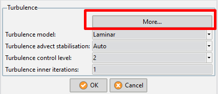
Advanced turbulence options can be accessed by using the following option of the tree to open the Ransol module Advanced
data window:
Note
Remarks:
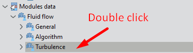
This option is not visible from the tree but it is visible when the turbulence panel is opened.
This panel is opened by double clicking on the ‘turbulence’ option
Fig. 1.12 With ‘Double click’ it is possible to open the ‘turbulence’ frame.
Fig. 1.13 ‘Turbulence’ frame where ‘More options’ are available.
The advanced options available in the contextual window are
detailed in what follows:
Fix Turbulence on Bodies: If Yes is selected, turbulence variables will have a fixed value,
given by the selected law of the wall on the bodies surfaces.
If No is selected, natural boundary condition will be applied.
Tvisco Min Ratio: Eddy viscosity ratio with the minimum of initial values of the eddy viscosity,
used to calculate the minimum admissible value.
Tvisco Max Ratio: Eddy viscosity ratio with the maximum of initial values of the eddy viscosity,
used to calculate the maximum admissible value (> 1.0).
Kenergy Min Ratio: Eddy kinetic energy (k) ratio with maximum of the initial values of k,
used to calculate the minimum admissible value.
Kenergy Max Ratio: Eddy kinetic energy (k) ratio with maximum of the initial values of k,
used to calculate the maximum admissible value.
Epsilon Min Ratio: Epsilon (ε) ratio with the maximum of initial values of ε,
used to calculate the minimum admissible value.
Epsilon Max Ratio: Epsilon (ε) ratio with the maximum of initial values of ε,
used to calculate the maximum admissible value.
Omega Min Ratio: Omega (ω) ratio with the maximum of initial values of ω,
used to calculate the minimum admissible value.
Omega Max Ratio: Omega (ω) ratio with the maximum of initial values of ω,
used to calculate the maximum admissible value (> 1.0).
K Tau Min Ratio: K Tau (kτ) ratio with the maximum of initial values of kτ,
used to calculate the minimum admissible value.
K Tau Max Ratio: K Tau (kτ) ratio with the maximum of initial values of kτ,
used to calculate the maximum admissible value.
Turbulence Control Level: Level of turbulence stabilisation control (0 means Off).
If instabilities are found in the eddy viscosity field, refine the mesh when possible,
reduce Time_Increment or increase this value. Note that too high values may cause overdiffusive eddy viscosity results.
Recommended value is 2.
EddyKEnergy Production Limit: Maximum ratio between the Eddy kinetic energy production and reaction term.
This limiter may prevent the unrealistic buildup of eddy viscosity in the stagnation region of the bodies.
Recommended value is 20.0.
Epsilon Production Limit: Maximum ratio between the Epsilon production and reaction term.
Epsilon Reaction Limit: Maximum ratio between the Epsilon reaction and production term.
Omega Production Limit: Maximum ratio between the Omega production and reaction term.
Omega Reaction Limit: Maximum ratio between the Omega reaction and production term.
EddyViscoT Production Limit: Maximum ratio between the Spallart-Almarax model production and reaction term.
EddyViscoT Reaction Limit: Maximum ratio between the SpallartAlmarax model reaction and production term.
Fluid Mesh Deformation: Mesh updating in fluid domain may be done by three different procedures:
Lagrangian update: Mesh deformation is performed following the velocity of the fluid.
The following equations must be entered in Fluid deformation increment:
OX: vx*dt
OY: vy*dt
OZ: vz*dt
ByBodies: Mesh deformation only takes into account the
movement of the defined bodies.
ByFunctions: Mesh deformation is performed following the values given in the Fluid Deformation Increment field.
ByAllData: Mesh deformation algorithm try to fulfil all the requirements
(movement of bodies, deformation given in Fluid Deformation Increment field and boundary conditions).
Update fluid mesh every (steps): Mesh updating in fluid domain in carried out every Update fluid mesh every (steps) steps.
If set to zero, the mesh deformation is just done before the first time step.
Fluid Deformation Increment: Functions defining fluid mesh deformation have to be inserted here.
These functions must define the deformation increment for every time step.
For example, a planar rotation around origin (0,0,0) may be defined by inserting the functions
xrot(w*dt), yrot(w*dt), 0.0, being w the angular velocity.
Note that if the geometry units and the deformation units are different,
since xrot and yrot are evaluated using internal units,
the returning values have to be multiplied by the unit conversion factor.
Solid Mesh Deformation: Mesh updating in solid domain may be done by three different procedures:
ByBodies: Mesh deformation only takes into account the movement of the defined bodies.
ByFunctions: Mesh deformation is performed following the values given in the Solid Deformation Increment field.
ByAllData: Mesh deformation algorithm try to fulfil all the requirements
(movement of bodies, deformation given in Solid Deformation Increment field and boundary conditions).
Update solid mesh every (steps): Mesh updating in solid domain in carried out every Update solid mesh every (steps) steps.
Solid Deformation Increment: Functions defining solid mesh deformation have to be inserted here.
These functions must define the deformation increment for every time step.
For example, a planar rotation around origin (0,0,0) may be defined by inserting the functions
xrot(w*dt), yrot(w*dt), 0.0, being w the angular velocity.
Note that if the geometry units and the deformation units are different,
since xrot and yrot are evaluated using internal units,
the returning values have to be multiplied by the unit conversion factor.
Movement stabilisation factor: This factor is used to increase stability of the body movement.
Higher values (>0.1) can produce compressibility effects which are necessary in the case of impact problems.
Increase of this parameter, should be followed by an increase of Pressure Inner Iterations value.
Temp. Advect Stabilisation: Order of the FIC advection stabilisation term in the temperature equation.
Three available options are Auto, 4th_Order and 2nd_Order.
Note
Remarks:
The 4th order term increases the accuracy of the solution and is recommended in most of the cases.
However in some problems it may cause instabilities.
Auto mode will automatically switch between 4th and 2nd order scheme,
depending on the smoothness of the solution.
Temp. Control Level: Level of control of instabilities (0 means Off).
If instabilities are found in the velocity field when using the 2nd_Order Temp.
Advect Stabilisation, first try to reduce Time Increment, then to increase this value.
Note that high values may cause over-diffusive results.
Temp. Inner Iterations: Number of iterations of the inner (nonlinear) temperature eq. solver
(performed every external iteration).
Temperature Norm: Temperature Euclidean norm used to check convergence in the non-linear iteration loop.
Prandtl Number: Prandtl number used to include turbulence effects in the temperature calculations.
Radiation model: model to be used in problems that involve heat transfer by radiation.
There are currently two different radiation models available in Tdyn CFD+HT,
P-1 and surface to surface (S2S) radiation models.
The P-1 radiation is the simplest case of the more general P-N model.
It is intended to be used in modelling problems that involve participating media,
since it includes the effect of scattering. On the other hand,
the S2S model is provided to take into account the radiation exchange in an
enclosure of gray-diffuse surfaces that depends on the size,
separation distance and orientation of the emitting surfaces.
It implies the usage of the view factor geometric function.
Elements per patch: this option only concerns the S2S heat transfer by ration model.
It determines the number of elements per patch to be used in the calculation of the view factor matrix.
A large number of elements per patch will reduce the computation time for the evaluation of
the view factor matrix at the expense of the accuracy.
Advect stabilisation: Order of the FIC advection stabilisation term in the variable equation.
Three available options are Auto, 4th_Order and 2nd_Order.
Note
Remarks:
The 4th order term increases the accuracy of the solution and is recommended in most of the cases.
However in some problems it may cause instabilities.
Auto mode will automatically switch between 4th and 2nd order scheme,
depending on the smoothness of the solution.
Control level: Level of control of instabilities (0 means Off).
If instabilities are found in the variable field when using the 2nd_OrderAdvect Stabilisation,
first try to reduce Time Increment, then to increase this value.
Note that high values may cause over-diffusive results.
Number of Phases: Set to One_Phase to just simulate the evolution of the primary phase
(mono-phase flow with free surface). This option is useful in many cases of water-air flows,
where the influence of the air movement in the water flow is negligible.
Two_Phases option will run the two phases flow algorithm.
Convergence norm: Euclidean norm used to check convergence in the non-linear iteration loop.
Solver Scheme: Set to Naval to increase the accuracy in
those problems where the pressure distribution is mainly hydrostatic
(it requires vertical coordinate to be parallel to Z axis).
Reinitialisation Every (Steps): In most of the cases, reinitialisation of the level set field
is not necessary to be done every time step. This option sets the number of time steps to wait to the next reinitialisation.
Boundary type: AdvancedOBC implements specific treatment of boundary conditions for odd level set equation in those
boundaries with fixed velocity conditions.
Mass conservation: If On is selected, additional conservation of primary phase is enforced.
If Fixed is selected the Mass increment per time step is defined in the next entry.
In those cases which the Mass increment is known, the accuracy of the results will be increases
selecting the Fixed option and inserting the correct value in the Mass increment entry.
Mass increment: Mass increment per time step used to apply additional volume conservation.
Units of the Mass increment: may be defined in the menu next to the Mass increment entry.
It is possible to define additional units by entering new dimensionally correct units in the box
(see Units Syntax section for further information).
This data group includes different entries required for the
thermal comfort module of Tdyn based on the Fanger’s method.
The Fanger’s method, through the calculation of the Predicted
Mean Vote (PMV), predicts the thermal comfort, and extends the
PMV to predict the proportion of dissatisfied people with the
environment in terms of their comfort vote, Predicted Percentage
Dissatisfied (PPD).
The PMV index predicts the mean response of a large group of
people according to the American Society of Heating, Refrigerating
and Air-Conditioning Engineers (ASHRAE) thermal sensation scale,
from -3 (cold) to +3 (hot), where 0 represents a neutral thermal
feeling.
Mean Radiant Temperature: the uniform temperature of an
imaginary enclosure in which the radiation from the occupant
equals the radiant heat transfer in the actual non-uniform enclosure.
Relative Humidity: a term used to describe the amount of water vapor
in a mixture of air and water vapor expressed as a percentage:
\[Hr [\%] = pv / ps · 100\]
where pv is the partial pressure of water vapor (H2O) and ps is the saturated vapor pressure of water.
Clothing Factor: insulation of clothes measured with the unit “clo”, where 1 clo = 0.155 m2K/W.
Metabolic Rate: human body heat production measured in the unit “met”, where 1 met = 58 W/mm2.
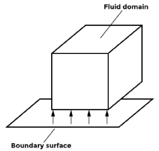
Conditions are all properties of a problem (except Materials) that can be
assigned to an entity, in order to define the basic boundary conditions of
a problem. Conditions should be used to define inflow and outflow boundary conditions,
symmetry or far field conditions, as well as complex boundary conditions like
body wall type (i.e. law of the wall) or free surface. In Tdyn CFD+HT conditions are
available through the Tdyn data tree that can be accessed by using the following
menu sequence:
In Tdyn CFD+HT conditions are available through the Tdyn data tree that
can be accessed by using the following menu sequence:
Tdyn Data > Conditions and initial data
If a mesh has already been generated, any change in the condition assignments,
requires meshing again to transfer these new conditions to the mesh.
If the conditions were changed and a new mesh was not generated, the user will be warned,
when the data for the analysis is being written.
Wall/Bodies boundaries allow the user to define special boundary conditions,
representing physical walls or bodies. The options available include analytical
Law of the Wall as well as body motion properties. These properties can be
assigned to lines (2D plane or 2D Axisymmetric), surfaces (3D) or boundary meshes.
Note
Remarks:
If any entity is defined as a Wall/Body the graphs of the reaction
forces on the fluid will be available in the postprocess of Tdyn CFD+HT.
If any entity is defined as a Wall/Body and any movement is enabled
(Mesh Deformation Analysis activated), the graphs of this movement
will be available in the postprocess of Tdyn CFD+HT.
In order to transfer Wall/Body data to the mesh, Meshing Criteria must be
fixed to Yes in the corresponding geometrical entities.
Note that this action is automatically done by Tdyn CFD+HT in most of the cases.
1.2.2.3.1.1.1. Options available in Wall Type page
Fluid/Solid Wall: Choose if the boundary condition is going to be applied
either to a Fluid or a Solid domain boundary.
BoundType: Type of the wall boundary. Several options are available:
InvisWall: Impose the slipping boundary condition (i.e. wall normal velocity component will be zero).
V_fixWall: Impose the null velocity condition on the boundary (i.e. velocity on the wall will be zero).
None_Wall: No conditions will be applied to the boundary. This boundary type
can be used to calculate forces on different parts of a body (in that case, the condition
will be superimposed on the standard body condition).
RoughWall: Law of the wall condition, taking wall roughness into account,
is applied at the wall distance δ. See Near wall-modelling chapter below.
The fluid stress (traction) given by the law of the wall at a wall
distance δ will be applied as boundary condition in the fluid solver.
The wall distance must be inserted in the field Delta (see below).
DeltaWall: Extended law of the wall condition is applied on the
boundary at the wall distance δ. See Near wall-modelling chapter below.
The fluid stress (traction) given by the law of the wall at a wall distance δ
will be applied as boundary condition in the fluid solver.
The wall distance must be inserted in the field Delta (see below).
YplusWall: Extended Law of the wall condition is applied on the boundary
at the non-dimensional wall distance y+. See Near wall-modelling chapter below.
The fluid stress (traction) given by the law of the wall at a non-dimensional
wall distance y+ will be applied as boundary condition in the fluid solver.
The non-dimensional wall distance must be inserted in the field Yplus (see below).
Cw_U2Wall: A traction given by Cw·V2, where Cwis a
constant and V the fluid velocity, is imposed on the boundary.
The constant Cwmust be inserted in the field Cw(see below).
ITTC Wall: Extended Law of the wall condition is applied on the boundary
at the non-dimensional wall distance y+. The fluid stress (traction) given by the
law of the wall at a non-dimensional wall distance y+ will be applied as
boundary condition in the fluid solver. This traction is corrected according to the
ITTC 57 friction law. The nondimensional wall distance must be inserted in the field Yplus (see below).
User Wall: Law of the wall formulation that can be defined by the user.
It requires explicit formulation of the wall traction (see below FTau Field),
eddy kinetic energy (see below KEnr Field) and the turbulence length scale (see below ELen Field).
Yplus: If YplusWall is selected, wall law assumption is taken up to the
non-dimensional wall distance y+ given here. The fluid stress (traction)
given by the law of the wall will be then applied as a boundary condition in the fluid solver.
See Near wall-modelling chapter below.
Delta: If DeltaWall or RoughWall is selected, wall law assumption is
taken up to the dimensional wall distance δ specified here. The fluid stress
(traction) given by the law of the wall will be then applied as a boundary condition
in the fluid solver. See Near wall-modelling chapter below.
Delta Units: Units of the dimensional wall distance δ given in the previous field.
Roughness: Roughness of the wall (only used if BoundType | RoughWall is selected).
Roughness Units: Units of the dimensional wall distance δ given in the previous field.
Cw: Constant used in the definition of BoundType | Cw_U2Wall.
VelX/Y/Z Field: Field used for defining the velocity profile on the boundary for V_fixBound BoundType.
VelN Field: Field used for defining the normal velocity profile on the boundary for VnfixBound BoundType.
FTau Field: Field of wall traction used in the definition of BoundType | User Wall.
It should be a explicit function of the variables used in Tdyn CFD+HT (see Function Syntax section for further information).
KEnr Field: Field of eddy kinetic energy used in the definition of BoundType | User Wall.
It should be a explicit function of the variables used in Tdyn CFD+HT
(see Function Syntax section for further information).
ELen Field: Field of turbulence length scale used in the definition of BoundType | User Wall.
It should be a explicit function of the variables used in Tdyn CFD+HT
(see Function Syntax section for further information).
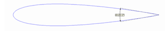
Sharp Angle: The slipping boundary condition for the velocity will be corrected
if any internal angle of this Fluid Body geometry is smaller than the one
inserted here (see the following figure). In those points, the boundary condition for the velocity is ignored.
This condition can be used for automatic correction of boundary conditions,
in those complex geometries with trailing edges, where the Fluid Body normal vector is undefined.
Fig. 1.14 Example of application of the Sharp Angle option
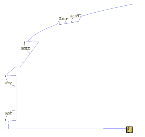
Line Fix Angle: Fix Velocity Direction boundary condition will be
automatically applied as boundary condition if an external angle of this Fluid Body
geometry is smaller than the one inserted here (see the following figure).
This condition should be used to automatically impose Fix Velocity Direction
boundary conditions, in those complex geometries with edges or significant dihedral angles,
where boundary conditions imposition by hand, may take too much time.
Note
Remarks:
In Tdyn CFD+HT 2D Plane a null velocity is imposed (instead of FixVelocity Directioncondition)
if an external angle of a Fluid Body is smaller than the one inserted here.
Fig. 1.15 Example of the places where the Line Fix Angle option could be useful.
SternC Angle: A control for stern of bodies (in the free surface transpiration problem)
is carried out. This control will be applied in those points of the floating line of the body,
where the angle between the normal and the velocity is greater that the value inserted here.
See Stern flow modelling in transpiration problem section.
Body Mass: Mass of the body. Units of the mass field may be
defined in the menu next to this entry. It is possible to define additional
units by entering new dimensionally correct units in the box
(see Units Syntax section for further information).
Note
Remarks:
If the check box next to the Body Mass entry is selected, mass of the body
will be estimated by Tdyn CFD+HT, based on a initial equilibrium of forces.
Body Mass entry will be available for all the modules of Tdyn CFD+HT,
not only when the Mesh Deformation Analysis is activated.
Center of Gravity: Vector giving the center of gravity of the body.
Units of the center of gravity may be defined in the units section of the data tree.
Tdyn Data > Simulation data > Units > Geometry units
Note
Remarks:
Center of Gravity entry will be available for all the modules of Tdyn CFD+HT,
not only when the Mesh Deformation Analysis is activated.
Center of Gravity can be defined by a time dependant function.
Center of Gravity position will be automatically updated with the movement of the Wall/Body.
Radi-us/-i of Gyration: Vector giving the radii of gyration of the body.
Units of the radii of gyration may be defined in the units section of the data tree .
Tdyn Data > Simulation data > Units > Geometry units
Displacement Options: For every displacement degree of freedom there
exists four possible options:
Off: the corresponding degree of freedom is disabled (movement is not allowed).
On: the corresponding degree of freedom is enables (movement is allowed).
If the value inserted in the corresponding Displacement Values field is
different from zero for t = 0, this value will be used to define an
initial movement of the body.
Fix: the corresponding degree of freedom is fixed to the time
dependant function given by the Displacement Values field (movement is prescribed).
This function is useful to impose rigid body motions.
Field: the corresponding degree of freedom is fixed to the generic function given
by the Displacement Values field (movement is prescribed).
This function is useful to impose body deformations.
Displacement Values: For every displacement degree of freedom, this vector
gives the total displacement of the body. The corresponding fields will
only be available if the Displacement Options field is selected as Fix.
Units of the displacement values vector may be defined in units section of the data tree:
Tdyn Data > Simulation data > Units > Geometry units
Rotation Options: For every rotational degree of freedom there exists three possible options:
Off: the corresponding degree of freedom is disabled (rotation is not allowed).
On: the corresponding degree of freedom is enables (rotation is allowed).
If the value inserted in the corresponding Rotation Values field is different from zero
for t = 0, this value will be used to define an initial movement of the body.
Fix: the corresponding degree of freedom is fixed to the value given by the
Rotation Values field (rotation is prescribed). This function is useful to impose rigid body motions.
Rotation Values: For every rotational degree of freedom, this vector gives the total rotation of the body.
The corresponding fields will only be available if the Rotation Options field is selected as Fix.
External Forces : This vector defines the additional external forces (gravity forces are not included)
acting on the center of gravity of the body.
External Moments: This vector defines the additional external moments
acting on the center of gravity of the body.
Relaxation factor: This factor is used to increase stability of the body movement.
The evaluation of the forces is relaxed, by averaging the previous and current value.
Recommended value is 0.25.
Damping factor: Damping added to the movement of the body.
If the objective of the analysis is the steady state,
it is recommended to increase the value of this factor
(recommended value in those cases is 0.75).
Inlet boundary condition is designed to represent a flow inlet. Use if the
boundary condition is going to be applied either to a Fluid or a Solid entity.
Inlet of: determines wether the inlet boundary condition corresponds to a fluid or a solid.
Boundary Type: Type of inlet boundary. Three options are available:
Inlet Velc: Allows defining a velocity profile on the boundary.
This profile is defined by inserting the velocity components in the fields VelX_Field, VelY_Field and VelZ_Field.
Inlet VelN: Allows defining the normal velocity on the boundary,
while tangential velocity is fixed to zero. This profile is defined
by inserting the normal velocity component in the field VelN_Field.
Inlet Pres: Allows defining a pressure field on the inlet boundary.
Outlet boundary condition is designed to represent a flow outlet.
Use if the boundary condition is going to be applied either to a Fluid or a Solid entity.
Outlet of: determines wether the outlet boundary condition corresponds to a fluid or a solid.
Boundary Type: Type of outlet boundary. Two options are available:
OutletPres: Pressure field is defined at the outlet boundary.
OutletNewm: A Newmann boundary condition on the velocity (null derivative) is defined at the outlet boundary.
This condition is assigned to geometrical/mesh entities or layers and is used to fix the pressure at the given value.
Note
Remarks:
When the selected flow model is PrCompressible (compressible based on pressure) both pressure and
density are prescribed when this condition is applied.
Fields: Pressure value: value (real) of the pressure.
Note
Remarks:
For most of the problems it is strongly recommended to fix the pressure in at least one point of the domain.
When the pressure is not specified in the analysis either directly or indirectly,
no reference for the pressure exists, and the resulting distribution can only be used with relative values.
The pressure can be specified at a far field boundary (i.e. at the outflow boundary of the domain,
when the boundary is far enough from the region of interest).
The pressure can also be specified at the inlet boundary. If the conditions at inlet are not well known,
it is effective to move the boundary as far from the region of interest as possible.
When the selected flow model is PrCompressible (compressible based on pressure) both pressure and
density are prescribed when this condition is applied.
This condition is assigned to geometrical/mesh entities and layers and is
used to specify the pressure at the value given by the pressure entry of the
conditional data (only if the Pressure FuncCond data field is greater than 0):
Tdyn Data > Conditions and initial data > Conditional data > PressureFuncCond
If the evaluation of the Pressure FuncCond field results in a value less than 0,
the boundary conditions will not be applied. If the value is 0, the boundary
condition will be applied only if it was applied in the previous time step.
Note
Remarks:
When the selected flow model is PrCompressible (compressible based on pressure)
both pressure and density are prescribed when this condition is applied.
When ConditionalPressure condition is assigned, Pressure Field entry is used both
for defining initial values (t = 0) when starting calculation and for evaluating the assigned
condition the rest of time steps.
Entries of Conditional data may be defined by functions (see Function Syntax section).
Pressure FuncCondand Pressure Field entries are common for every
Conditional Pressure condition and can only be
modified in the Conditional data of the Fluid Flow conditions.
In most of the problems, it is recommended to fix the pressure in at least one point of the domain.
When the pressure is not specified in the analysis either directly or indirectly,
no reference for the pressure exists, and the resulting distribution can only be used with relative values.
Sometimes the pressure is specified at a far field boundary
(i.e. at the outflow boundary of the domain,
when the boundary is far enough from the region of interest).
Sometimes the pressure is specified also at the inlet boundary.
If the conditions at inlet are not well known, it is effective to move
the boundary as far from the region of interest as possible.
This condition is assigned to geometrical/mesh entities and is used to fix the
pressure at the value given by the Pressure Field entry of the initial and field
data conditions in the data tree:
Tdyn Data > Conditions and initial data > Initial and Conditional data > Pressure Field
Note
Remarks:
When the selected flow model is PrCompressible (compressible based on pressure)
both pressure and density are prescribed when this condition is applied.
Fix Initial: The pressure will be fixed to the initial value (evaluated at t=0)
of the function inserted in the Pressure Field entry of the Initial and Field
data conditions in the tree. Pressure Field entry is evaluated at the initial
step (t=0) and pressure is fixed to the resulting value for the rest of the execution.
Fix Field: The pressure will be fixed to the value (for every time step) of the function
inserted in the Pressure Field of the Initial and Field data conditions in the tree.
Pressure Field entry is evaluated every step and pressure is fixed to the resulting value.
Note
Remarks:
In most of the problems, it is recommended to fix the pressure in
at least one point of the domain. When the pressure is not specified
in the analysis either directly or indirectly, no reference for the
pressure exists, and the resulting distribution can only be used with relative values.
When Pressure Field condition is assigned, Pressure Field entry
is used both for defining initial values (t = 0) when starting calculation
and for evaluating the assigned condition the rest of time steps.
Pressure Field value is common for every Pressure Field condition
and can only be modified in the Initial and Field data conditions in the tree.
Sometimes the pressure is specified at a far field boundary
(i.e. at the outflow boundary of the domain, when the boundary is far enough from the region of interest).
Sometimes the pressure is specified also at the inlet boundary.
If the conditions at inlet are not well known, it is effective to move
the boundary as far from the region of interest as possible.
This condition allows a definition of transient boundary conditions
for the pressure. The analytical functions defining transient boundary
conditions will be specified in the corresponding function inserted
in the Pressure Field entry of the Initial and Field data conditions in the tree.
If the boundary conditions for the pressure are steady, this condition can be substituted
by the Fix Pressure condition. The only difference between these two options
in this case is, that when using Pressure Field, the value of the
fixed pressure can be changed automatically in every entity by updating
the corresponding function inserted in the Pressure Field entry of the
Initial and Field data conditions in the tree.
Entries of the Initial and Field data conditions may be defined by functions
(see Function Syntax section).
This condition is assigned to geometrical/mesh entities or layers and is used to
fix the velocity at the given value.
X Component: Value (real) of the OX component of the velocity.
Fix X: Only if marked the OX component of the velocity will be fixed.
Y Component: Value (real) of the OY component of the velocity.
Fix Y: Only if marked the OY component of the velocity will be fixed.
Z Component: Value (real) of the OZ component of the velocity.
Fix Z: Only if marked the OZ component of the velocity will be fixed.
Note
Remarks:
The velocity has to be prescribed at the inlet boundary.
If the conditions at inlet are not well known, it is effective to move the
boundary as far from the region of interest as possible.
This condition is assigned to geometrical/mesh entities and layers and
is used to specify the velocity at the value given by the corresponding
Velocity X/Y/Z Field entries of the Conditional data conditions in the tree
(only if the given conditional data field is greater than 0):
Tdyn Data > Conditions and initial data > Initial and Conditional data > Conditional data > Velocity X/Y/Z FuncCond
If the evaluation of the corresponding Velocity X/Y/Z FuncCond field results
in a value less than 0, the boundary conditions will not be applied. If the value is 0,
the boundary condition will be applied only if it was applied in the previous time step.
Note
Remarks:
When Conditional Velocity condition is assigned, Velocity X/Y/Z Field
entries are used both for defining initial values (t = 0) when starting
calculation and for evaluating the assigned condition the rest of time steps.
Entries of the Conditional data may be defined by functions (see Function Syntax section).
Velocity X/Y/Z FuncCond entries are common for every Conditional Velocity
condition and can only be modified in the Conditional data.
The velocity has to be prescribed at every inlet boundary. If the conditions
at inlet are not well known, it is effective to move the boundary as far
from the region of interest as possible.
This condition is assigned to geometrical/mesh entities and layers and is
used to specify the velocity at the value given by the corresponding functions
of the Initial and Field data section of the data tree:
Tdyn Data > Conditions and initial data > Initial and Conditional data > Initial and Field data
Note
Remarks:
Entries of the Initial and Field data may be defined by functions (see Function Syntax section).
Fields:
Fix Initial X: The OX component of the velocity will be fixed to the initial
value (evaluated in t=0) of the corresponding function of the Initial and Field
data (Velocity X Field entry) only if the field is marked. Velocity X Field
is evaluated at the initial step (t=0) and velocity component is fixed to the resulting
value for the rest of the execution.
Fix Initial Y: The OY component of the velocity will be fixed to the initial value
(evaluated in t=0) of the corresponding function of the Initial and Field data
(Velocity Y Field entry) only if the field is marked. Velocity Y Field is evaluated
at the initial step (t=0) and velocity component is fixed to the resulting value for the
rest of the execution.
Fix Initial Z: The OZ component of the velocity will be fixed to the initial value
(evaluated in t=0) of the corresponding function of the Initial and Field data
(Velocity Z Field entry) only if the field is marked. Velocity Z Field is
evaluated at the initial step (t=0) and velocity component is fixed to the resulting value for the
rest of the execution.
Fix Field X: The OX component of the velocity will be fixed to the value
(for every time step) of the corresponding function of Initial and Field
data (Velocity X Field entry) only if the field is marked.
Velocity X Field is evaluated every step and the corresponding velocity
component is fixed to the resulting value.
Fix Field Y: The OY component of the velocity will be fixed to the value
(for every time step) of the corresponding function of the Initial and Field
data (Velocity Y Field entry) only if the field is marked.
Velocity Y Field is evaluated every step and the corresponding velocity
component is fixed to the resulting value.
Fix Field Z: The OZ component of the velocity will be fixed to the value
(for every time step) of the corresponding function of the Initial and Field
data (Velocity Z Field entry) only if the field is marked.
Velocity Z Field is evaluated every step and the corresponding velocity
component is fixed to the resulting value.
Note
Remarks:
The velocity has to be prescribed at every inlet boundary. If the conditions
at inlet are not well known, it is effective to move the boundary as far
from the region of interest as possible.
When Velocity Field condition is assigned, Velocity X/Y/Z Field
entries are used both for defining initial values (t = 0) when starting
calculation and for evaluating the assigned condition the rest of time steps.
This condition allows definitions of transient boundary conditions for the
velocity. The analytical functions defining transient boundary conditions
will be specified in the corresponding Initial and Field data
section of the data tree.
If the boundary conditions for the velocity are steady, this condition
can be substituted by the Fix Velocity condition. The only difference
between these two options in this case is, that when using the Velocity Field,
the value of the fixed velocity can be changed automatically in every entity
by updating the corresponding Initial and Field data of the Fluid Flow
conditions in the tree.
This condition is assigned to geometrical/mesh entities and layers and
is used to fix the turbulence variables for those turbulence models based
on the Reynolds extended analogy, at the initial (evaluated for t=0) value given
by the corresponding functions (EddyKEner Field and EddyLength Field) of the
Initial and Field data section of the data tree:
Tdyn Data > Conditions and initial data > Initial and Conditional data > Initial and Field data > EddyKEner field
Tdyn Data > Conditions and initial data > Initial and Conditional data > Initial and Field data > EddyLength field
Fields:
Fix: The turbulence will be fixed to the initial value (evaluated in t=0) of the
corresponding function of the Initial and Field data section the tree only if
this field is marked. EddyKEner Field and EddyLength Field give the value
of the eddy energy and turbulence length scale or mixing length
(see Turbulence modelling section), respectively.
Note
Remarks:
The turbulence variables have to be prescribed at every inlet boundary.
In those entities where all components of the velocity have been prescribed,
Tdyn CFD+HT automatically fixes all turbulence variables at the initial
(evaluated for t=0) value given in the EddyKEner Field and EddyLength Field
entries of the Initial and Field data section of the tree. Therefore,
assignment of this condition should not be necessary in most of the cases.
Fix Turbulence condition will only be useful for those turbulence
models based on Reynolds extended analogy (see Turbulence Modelling
section for further information)
This condition is assigned to geometrical/mesh entities and layers and makes
the program to ignore any specification on the velocity field.
Fields:
Free Velocity: The velocity will be removed only if this field is marked.
Note
Remarks:
This option allows the solver to accomplish the KuttaJukowsky condition.
In these cases the Remove Velocity condition will be assigned to the extreme
point of the tail of a profile. It is also possible to automatically correct
velocity impositions in these areas by using the Wall/Bodies options
(see Sharp Angle option).
This condition is assigned to geometrical/mesh entities and may be used to define the
direction of the velocity, according to the orientation of the skew system.
Fields:
Local Axes: Orientation of the Cartesian axes used to define the direction of the
component of the velocity vector. These can be local axes of the geometry
(-Automatic- option) or any user defined system.
Type: Axis of the Local Axes definition. The component of the velocity vector,
parallel to this axis, will be fixed to the given value.
The normal velocity component to a line or a surface can be fixed by selecting
Y_Axis or Z_Axis. To see the defined Local Axes, press the button Draw.
Note
Remarks:
Usually, the direction of the velocity has to be prescribed in some edges or
areas with strong geometrical changes of the geometry.
The direction of the velocity can be automatically imposed by using the Wall/Bodies options
(see Fix Angle option).
This condition is assigned to geometrical/mesh and is used to specify the
value of a component of the velocity vector.
Fields:
Local Axes: Orientation of the Cartesian axes used to define the direction of the
component of the velocity vector. These can be local axes of the geometry
(-Automatic- option) or any user defined system.
Type: Axis of the Local Axes definition. The component of the velocity vector,
parallel to this axis, will be fixed to the given value. The normal velocity component
to a line or a surface can be fixed by selecting Y_Axis or Z_Axis.
To see the defined Local Axes, press the button Draw.
Value: Value of the component of the velocity in the direction given by Type axis.
Note
Remarks:
This option is used to prescribe slipping boundary conditions on a velocity field.
Since the normal vector is sometimes undefined in some complex areas (i.e. dihedral angles) of the geometry,
in some cases it is better to use the Wall/Bodies options instead.
This condition is assigned to geometrical/mesh entities and layers and is
used to fix the temperature in a geometrical entity or layer to the given value.
This condition is assigned to geometrical/mesh entities and layers and is
used to fix the temperature to the value given by the function inserted in the
Temperature FuncCond entry of the Conditional Data section of the tree:
Tdyn Data > Conditions and initial data > Initial and field data > Conditional data > Temperature FuncCond
Fields:
Fix Initial: The temperature will be fixed to the initial value
(evaluated in t=0) of the function inserted in the Temperature FuncCond
entry of the Conditional Data only if the field is marked.
Temperature Field is evaluated initial step (t=0) and temperature is fixed to
the resulting value for the rest of the execution.
Fix Field: The temperature will be fixed to the value (for every time step)
of the function inserted in the Temperature FuncCond entry of the Conditional Data.
Temperature FuncCond entry is evaluated every step and temperature is fixed to the resulting value.
Note
Remarks:
This condition allows definitions of transient boundary conditions for temperature.
The analytical functions defining transient boundary conditions will be specified in
the Temperature FuncCond entry of the Conditional Data in Heat Transfer Conditions entry of the tree.
If the boundary conditions for the temperature are steady, this condition can be substituted by the Fix Temperature
condition. The only difference between these two options in this case is, that when using the Temperature Field,
the value of the fixed temperature can be changed automatically in every entity by updating the Temperature Field
entry of the Conditional Data.
When Temperature Field condition is assigned, Temperature Field entry is used both for defining
initial values (t = 0) when starting calculation and for evaluating the assigned condition the rest of time steps.
This condition is assigned to geometrical/mesh entities and layers and is
used to fix the temperature at the value given by the function inserted in the
Temperature Field entry of the Initial and Field Data section of the tree:
Conditions and Initial data ► Initial and Conditional data ►
Initial and Field data ► Temperature field
Tdyn Data > Conditions and initial data > Initial and field data > Initial and Field data > Temperature field
Fields:
Fix Initial: The temperature will be fixed to the initial value
(evaluated in t=0) of the function inserted in the Temperature Field entry of Initial and Field Data only if the field is marked.
Temperature Field is evaluated initial step (t=0) and temperature is fixed to the resulting value for the rest of the execution.
Fix Field: The temperature will be fixed to the value (for every time step)
of the function inserted in the Temperature Field entry of Initial and Field Data.
Temperature Field entry is evaluated every step and temperature is fixed to the resulting value.
Remarks:
This condition allows definitions of transient boundary conditions for temperature.
The analytical functions defining transient boundary conditions will be specified in
the Temperature Field entry of Initial and Field Data.
If the boundary conditions for the temperature are steady, this condition can be substituted
by the Fix Temperature condition. The only difference between these two options
in this case is, that when using the Temperature Field, the value of the fixed
temperature can be changed automatically in every entity by updating the
Temperature Field entry of Initial and Field Data.
When Temperature Field condition is assigned, Temperature Field entry is
used both for defining initial values (t = 0) when starting calculation and
for evaluating the assigned condition the rest of time steps.
Heat Flux: Heat flow (power) entering to domain through this
Fluid/Solid Boundary. It may be a constant or a function. Units of the
heat flux field may be defined in the menu next to this entry.
It is possible to define additional units by entering new dimensionally
correct units in the box (see Units Syntax section for further information).
Note that positive values mean heat flow entering the domain.
Reactive Heat Flux: Factor of the reactive term of the heat flow (power)
entering to the domain through this Fluid/Solid Boundary.
The value here inserted will be multiplied by the current temperature
to obtain the heat flow. It may be a constant or a function. Units of the reactive
heat flux field may be defined in the menu next to this entry. It is possible
to define additional units by entering new dimensionally correct units in the box
(see Units Syntax section for further information)
Note
Remarks:
Convection heat transfer may be simulated by inserting the function q - h·(Tm-To)
in the field Heat Flux, being q a defined heat flow, h the transmission coefficient and
To the external temperature. However it is recommended to split this flow in two terms,
constant flow q +h·To that should be inserted in the Heat Flow field and the coefficient
of the temperature dependent term h, that should be entered in Reactive Heat Flux field.
Emissivity: value of the emissivity to be used for the surfaces
assigned to the corresponding radiation flux condition. In heat radiation problems
this quantity measures the effectiveness of a material surface in emitting
energy as thermal radiation. Quantitatively, emissivity is the ratio of
the thermal radiation from a surface to the radiation from an ideal black
surface at the same temperature as given by the Stefan-Boltzmann law.
It must be a real value between 0.0 and 1.0
Wall temperature: value of temperature for the surfaces assigned to the
corresponding radiation flux condition when using the P-1 radiation model.
This condition is assigned to geometrical/mesh entities and layers and
is used to fix the value of the concentration of species (substances) at the given value.
Fields:
Species Name: Name of the species (see Edit Species description in section Materials) which concentration is to be fixed.
Concentration: Value of the concentration of the species.
Note
Remarks:
The value of the concentration of every species should be prescribed at every inlet boundary.
This condition is assigned to geometrical/mesh entities and layers and
is used to specify the concentration of species to the value given by the Concentration Field
entry of the Initial and Conditional data section of the corresponding
specie definition that is done within the Materials section of the data tree
(only if the corredponding Concentration Field data is greater than 0):
Materials ► Edit species ► Specie name ► Initial and
Conditional
Tdyn Data > Conditions and initial data > Initial and field data > Initial and Field data > Temperature field
If the evaluation of the Concentration Field results in a value less than 0,
the boundary conditions will not be applied. If the value is 0,
the boundary condition will be applied only if it was applied in the previous time step.
Note
Remarks:
Entries of Initial and Conditional data may be defined by functions (see Function Syntax section).
Concentration Field and Species Conditional entries of a given specie definition are common for every
Conditional Concentration condition and can only be modified in the Initial and Conditional
data section of the specie definition.
When Conditional Concentration condition is assigned, Conc. Field entry is used both for defining
initial values (t = 0) when starting calculation and for evaluating the assigned condition
the rest of time steps.
This condition is assigned to geometrical/mesh entities and is used to fix the
concentration of species to the value given by the Concentration Field entry
of the Initial and Conditional data section of the corresponding specie
definition beneath the Materials section:
Tdyn Data > Materials > Edit species > Specie name > Initial and Conditional
Fields:
Specie: Name of the species (see Edit Species description in section Materials)
whose concentration is going to be fixed.
Fix Initial: The concentration of the species will be fixed to the
initial value (evaluated in t=0) of the function inserted in the
Concentration Field entry of the Initial and Conditional data section
of the specie definition. Concentration Field entry is evaluated at
the initial step (t=0) and concentration is fixed to the resulting value
for the rest of the execution.
Fix Field: The concentration will be fixed to the value (for every time step)
of the function inserted in the Concentration Field entry of the
Initial and Conditional data section of the specie definition.
Concentration Field entry is evaluated every step and concentration is fixed to the resulting value.
Note
Remarks: The value of the concentration of each specie should be
prescribed at every inlet boundary.
This condition allows definitions of transient boundary conditions for concentration.
The analytical functions defining transient boundary conditions will be
specified in the Concentration Fiel entry of the Initial and Conditional
data section of the specie definition.
If the boundary conditions for the concentration are steady, this condition can be
substituted by the Fix Concentration condition. The only difference between
these two options in this case is, that when using the Concentration Field,
the value of the fixed concentration can be changed automatically in every
entity by updating the Concentration Field entry of the Initial and Conditional
data section of the specie definition.
When Concentration Field condition is assigned, Concentration Field
entry is used both for defining initial values (t = 0) when starting
calculation and for evaluating the assigned condition the rest of time steps.
Advect Flux Solids/Fluids allows to select among the different created
species list, to assign to them a flux through a certain boundary.
Fields:
Specie: name of the specie to which the advect flux condition will refer to.
SpecieFlux: Flow of the species entering to the domain through this
Fluid/Solid Body. It may be a constant or a function. Units of the flux
specie field may be defined in the menu next to this entry. It is possible
to define additional units by entering new dimensionally correct units in
the box (see Units Syntax section for further information).
Reactive Specie Flux: Factor of the reactive term of the flow of the species
entering to the domain through this Fluid/Solid Body. The value here inserted
will be multiplied by the current species concentration to obtain the heat flow.
It may be a constant or a function. Units of the reactive flux specie field may
be defined in the menu next to this entry. It is possible to define additional
units by entering new dimensionally correct units in the box (see Units Syntax
section for further information).
Note
Remarks: Entering flow of species of the form h·sp1 should be
inserted in the Reactive Specie Flux field as h. Note that positive values
means flow entering in the domain.
This condition is assigned to geometrical/mesh entities and layers and
is used to specify the value of a variable at the value given by the Variable Field
entry of the Initial and Conditional data section of the variable
definition in the Materials section of the tree (only if the evaluation of the
function defined in Variable field is greater than 0):
Tdyn Data > Materials > Edit PDEs variables > Variable > Initial and Conditional
If the evaluation of the Variable field results in a value less than 0, the
boundary conditions will not be applied. If the value is 0, the boundary condition
will be applied only if it was applied in the previous time step.
Note
Remarks: Entries of the Initial and Conditional data section
of the variable definition (within the Materials section) may be
defined by functions (see Function Syntax section). Variable field and
Variable FuncCond entries are common for every Conditional Variable
condition and can only be modified in the Initial and Conditional
section of the variable definition.
When Conditional Variable condition is assigned the Variable field
entry is used for defining both initial values (t = 0) when starting
calculation and for evaluating the assigned condition the rest of time steps.
This condition is assigned to geometrical/mesh entities and is used to fix
the value of a variable to the value given by the Variable Field entry of the
Initial and Conditional data section of the corresponding variable definition
(within the Materials section of the data tree):
Tdyn Data > Materials > Edit PDEs variables > Variable > Initial and Conditional
Fields:
Variable: Name of the variable (see Edit PDEs variables description
in section Materials) which value is to be fixed.
Fix Initial: The variable will be fixed to the initial value (evaluated in t=0)
of the function inserted in the Variable Field entry of the Initial and Conditional
data section of the variable definition. Variable Field entry is evaluated
at the initial step (t=0) and the variable is fixed to the resulting value for
the rest of the execution.
Fix Field: The variable will be fixed to the value (for every time step)
of the function inserted in the Variable Field entry of the Initial and Conditional
data section of the variable definition. Variable Field entry is evaluated every step and
Variable is fixed to the resulting value.
Note
Remarks: The value of the variable should be prescribed at every inlet boundary.
This condition allows definitions of transient boundary conditions
for variables. The analytical functions defining transient boundary
conditions will be specified in the Variable Field entry of the
Initial and Conditional data section of the variable definition.
If the boundary conditions for the variable are steady, this condition can be
substituted by the Fix Variable condition. The only difference between these two
options in this case is, that when using the Variable Field condition, the value
of the fixed variable can be easily updated in every entity by changing the
Variable Field entry of the Initial and Conditional data section of
the variable definition.
When Variable Field condition is assigned Variable Field entry is
used both for defining initial values (t = 0) when starting calculation
and for evaluating the assigned condition the rest of time steps.
PDEs Variables Flux Solids/Fluids allows to select among the list of created variables,
to assign to them a flux through a certain boundary.
Fields:
Variable Flux: Flow of the variable entering to the domain through this
Fluid/Solid Body. It may be a constant or a function. Units of the flux phi
field may be defined in the menu next to this entry. It is possible to define
additional units by entering new dimensionally correct units in the box (see Units
Syntax section for further information).
Reactive Variable Flux: Factor of the reactive term of the flow of the species
entering to the domain through this Fluid/Solid Body. The value here inserted
will be multiplied by the current variable concentration to obtain the heat flow.
It may be a constant or a function. Units of the reactive flux phi field may be defined
in the menu next to this entry. It is possible to define additional units by
entering new dimensionally correct units in the box (see Units Syntax section for further information).
Note
Remarks: Entering flow of the variable of the form h·ph1 should be
inserted in the Reactive Variable Flux field as h. Note that positive values
means flow entering in the domain.
This condition is assigned to geometrical/mesh entities and layers. It is used
to fix the value of the mesh deformation to zero or to the value given in
the Fluid Deformation Increment OX/OY/OZ fields in the Mesh deformation
section of the data tree. See the following Modules Data section of the tree:
Tdyn Data > Modules data > Mesh deformation
Fields:
Type: Type of mesh deformation. If Fix Field is selected, imposed mesh
deformation will be defined by Fluid/Solid Deformation Increment OX/OY/OZ
fields (specified within the Modules data).
If Fix Null is selected, mesh deformation is forced to be zero.
Finally, if No Fix is selected, any other imposition on the mesh
deformation field is ignored.
Note
Remarks: The type of Fluid mesh deformation to be imposed may be
defined in the Modules Data section of the tree:
This condition is assigned to geometrical/mesh entities. It is used to
fix the value of the fluid flow on the selected entity to the value of the
mesh deformation velocity.
Conditions and Initial data ► Mesh deformation ► Fix mesh
velocity
Tdyn Data > Conditions and Initial data > Mesh deformation > Fix mesh velocity
Fields:
Fix X: mark this field in order to fix the X velocity component of the
fluid flow to the value provided by the X component of the mesh deformation velocity.
Fix Y: mark this field in order to fix the Y velocity component of the
fluid flow to the value provided by the Y component of the mesh deformation velocity.
Fix Z: mark this field in order to fix the Z velocity component of the
fluid flow to the value provided by the Z component of the mesh deformation velocity.
This condition is assigned to geometrical/mesh entities and is used to fix
the value of the level set function to the value given by the OddLevelSet field
entry of the Initial and Field data section of the tree:
Tdyn Data > Conditions and Initial data > Initial and Conditional data > Initial and Field data
Fields:
Fix Initial: The level set function will be fixed to the initial value
(evaluated in t=0) of the function inserted in the OddLevelSet field entry
of the Initial and Field data section of the tree.
OddLevelSet field entry is evaluated at the initial step (t=0) and level
set function is fixed to the resulting value for the rest of the execution.
Fix Field: The level set function will be fixed to the value
(evaluated every time step) of the function inserted in the
OddLevelSet Field entry of Initial and Field data section of the tree.
OddLevelSet field entry is evaluated every time step and level set
function is fixed to the resulting value.
Note
Remarks: The value of the level set function should be prescribed at
every inlet boundary.
This condition allows definitions of transient boundary conditions
for level set function. The analytical functions defining transient
boundary conditions will be specified in the OddLevelSet field entry
of Initial and Field data.
If the boundary conditions for the variable are steady, this condition
can be substituted by the Fix ODDLS condition.The only difference
between these two options in this case is, that when using the
ODDLS Field the value of the fixed variable can be easily updated
in every entity by changing the OddLevelSet field of Initial and Field data.
When ODDLS Field condition is assigned, OddLevelSet field entry
is used both for defining initial values (t = 0) when starting
calculation and for evaluating the assigned condition the rest of time steps.
This condition is assigned to geometrical/mesh entities and layers and
is used to specify the value of the level set function at the value given by
the OddLevelSet FuncCond entry of the Conditional data section of the tree
(only if the OddLevelSet FuncCond data field is greater than 0):
Tdyn Data > Conditions and Initial data > Initial and Conditional data > Conditional data > OddLevelSet FuncCond
If the evaluation of the OddLevelSet FuncCond field results in a value less than 0,
the boundary conditions will not be applied. If the value is 0, the boundary condition
will be applied only if it was applied in the previous time step.
Note
Remarks: Entries of Cond. Data may be defined by functions
(see Function Syntax section).
OddLevelSet FuncCond and OddLevelSet Field entries are common for every
Conditional ODDLS condition and can only be modified in Cond. Data.
When Conditional ODDLS condition is assigned, OddLevelSet Field entry
is used both for defining initial values (t = 0) when starting calculation
and for evaluating the assigned condition the rest of time steps.
This condition is assigned to geometrical/mesh entities and layers.
It is used to fix the value of the wave elevation to its initial value.
The initial value is the difference between the OZ coordinate of the point
and the reference height of the free surface. See the following Modules data section of the tree:
Tdyn Data > Modules data > Fluid flow > General > Pressure reference location
Fields:
Fix: The wave elevation will be fixed to its initial value only if this field is marked.
Note
Remarks: This option is effective in the stern of some geometries to
keep the stability of the free surface. In most of the cases it can be
automatically imposed by using the Wall/Body options
(see Stern C Angle option and Stern flow modelling in transpiration problem section).
Free Surface boundary conditions identify a free surface boundary of a
fluid in the analysis. These properties can be assigned to surfaces (3D).
Note
Remarks: Free Surface boundary condition is only available
if the Free Surface (Transpiration) Analysis is activated.
In order to transfer Free Surface data to the mesh, Meshing
Criteria must be fixed to Yes in the corresponding geometrical entities.
Note that this action is automatically done by Tdyn CFD+HT in most of the cases.
General fields:
Time Integration: Time integration scheme used in the solution process of
the free surface problem. The following options are available:
Adams_Bashforth_2: Explicit 2nd order Adams Bashforth scheme.
Stabilised_FIC: Time stabilised FIC scheme.
Backward_Euler: Implicit 1st order Backward Euler scheme.
Forward_Euler: Explicit 1st order Forward Euler scheme.
Crank_Nicolson: Implicit 2nd order Crank-Nicolson scheme.
Length: Characteristic length of the free surface problem
(i.e. length of the Fluid Body).
Damping length: Relative damping length (total damping length is given
by Damping Length x Length) to be used in this free surface calculation.
The damping of the generated waves starts at a total damping length distance
from the outlet of the free surface.
Note
Remarks: In most of the cases cases it is necessary to damp the wave
elevation in order not to find bouncing effects in the boundaries.
Damping factor: Factor that controls the damping effect.
Advanced fields:
Time factor: Time integration security factor to be used in the
explicit integration (i.e. Adams_Bashforth_2, Stabilised_FIC and
Forward_Euler schemes) of this free surface.
Step factor: Time step ratio between free surface and fluid solver.
It is possible to accelerate convergence by increasing this ratio,
but may cause instability in the integration scheme. If chosen Time
Increment is too high, reduce this value to achieve convergence.
Note
Remarks: Note that solutions with Step factor != 1 will only
give realistic results for the steady state.
Advect_Stabilisation: The order of the FIC advection stabilisation term
in the free surface equation. Two options are available 4th_Order and 2nd_Order.
Note
Remarks: The 4th order term increases the accuracy of the solution
and is recommended in most of the cases, but in some problems may
appear instabilities.
StabTau_MinRatio: Minimum admissible ratio (τ/dt, being dt the time increment)
for the stabilisation parameter τ.
Note
Remarks: Advection stabilisation term is proportional to the
parameter τ. In most of the cases, the minimum value of this parameter
should not be fixed (i.e. τ/dt = 0.0), otherwise oscillations may appear.
Solid-Solid Contact boundaries identify a contact with continuity of the
corresponding field between two disjoint solid domains.
Contact properties can be defined and assigned to lines (2D Plane & 2D
Asisymmetric analysis) or surfaces (3D analysis) or boundary meshes.
Three contact types are available:
Interpolating contact: this type of contact concerns the tradicional
contact algorithm. Contact surfaces must be coincident, although resulting
contact meshes may be different in each side.
Distance contact: this type of contact allows to correlate the results between
two surfaces which are not truly in contact and that can be even moving apart from each other.
Periodic contact: this type of contact is used to enforce periodic
boundary conditions. When this type of contact is selected, X/Y/Z Distance
fields become active so that distance functions can be defined in order to specify the
periodicity of the contact.
1.2.2.4.1.1. Options available in Fluid Flow module
Activate contact: if this check button is activated, the contact
algorithm will enforce continuity in both, velocity and pressure, across or between solid domains.
Activate contact (only velocity): if this check button is activated, the
contact algorithm will enforce continuity only in velocity across or between solid domains.
Note that these two options are mutually exclusive.
1.2.2.4.1.2. Options available in Heat Transfer module
Activate contact: thermal contact is only active if the checkbutton is selected.
If the checkbutton is not selected, thermal resistance is assumed to be infinite.
Thermal resistance: thermal resistance of the temperature contact between solid materials.
If thermal resistance is null, contact is perfect. Thermal resistance R of an homogeneous
layer of a solid material, can be calculated as R = e / k, being e the thickness of the layer,
and k the thermal conductivity of the material.
1.2.2.4.1.3. Options available in PDE’s solver module
Active variable: individual check buttons are available for each defined generic variable.
The check button must be selected in order to activate the contact for the corresponding variable.
If a check button is not selected, an infinite resistance is assumed to exist for that particular variable.
Resistance: Resistance term (R), defining variables flow through the
contact as dφ/dn=R·(φ1-φ2) being φ1 andφ2 the concentration (of the corresponding variables)
in domains 1 and 2 respectively. If resistance is null, contact is perfect.
1.2.2.4.1.4. Options available in Mesh Deformation module
Activate Contact: Select to activate the contact between two solid
domains for the mesh deformation algorithm. Such and option
is only effective if the ByBodies mesh deformation type has been
selected in the data tree as follows:
Tdyn Data > Modules data > Mesh deformation > Fluid mesh deformation > ByBodies
Fluid-Fluid Contact boundaries identify a contact with continuity of
the corresponding field between two disjoint fluid domains. Contact properties
can be defined and assigned to lines (2D Plane & 2D Asisymmetric analysis)
or surfaces (3D analysis) or boundary meshes. Three contact types are available:
Interpolating contact: this type of contact concerns the tradicional
contact algorithm. Contact surfaces must be coincident, although resulting
contact meshes may be different in each side.
Distance contact: this type of contact allows to correlate the results
between two surfaces which are not truly in contact and that can be even
moving apart from each other.
Periodic contact: this type of contact is used to enforce periodic boundary
conditions. When this type of contact is selected, X/Y/Z Distance fields
become active so that distance functions can be defined in order to specify the
periodicity of the contact.
1.2.2.4.2.1. Options available in Fluid Flow module
Activate contact: if this check button is activated, the contact
algorithm will enforce continuity in both, velocity and pressure, across or
between fluid domains.
Activate contact (only velocity): if this check button is activated,
the contact algorithm will enforce continuity only in velocity across
or between fluid domains.
Note that these two options are mutually exclusive.
1.2.2.4.2.2. Options available in Heat Transfer module
Activate contact: thermal contact is only active if the checkbutton
is selected. If the check-button is not selected, thermal resistance is
assumed to be infinite.
Thermal resistance: thermal resistance of the temperature contact between
fluid materials. If thermal resistance is null, contact is perfect.
Thermal resistance R of an homogeneous layer of a solid material, can be
calculated as R = e / k, being e the thickness of the layer, and k the thermal
conductivity of the material.
1.2.2.4.2.3. Options available in Species Advection module
Active species: individual check buttons are available for each existing specie.
The check button must be selected in order to activate the contact for the
corresponding specie. If a check button is not selected, an infinite resistance
is assumed to exist for that particular specie.
Resistance: Resistance term (R), defining species flow through the contact
as dφ/dn=R·(c1-c2) being c1 and c2 the concentration (of the corresponding species)
in domains 1 and 2 respectively. If resistance is null, contact is perfect.
1.2.2.4.2.4. Options available in PDE’s solver module
Active variable: individual check buttons are available for each
defined generic variable. The check button must be selected in order to activate
the contact for the corresponding variable. If a check button is not selected,
an infinite resistance is assumed to exist for that particular variable.
Resistance: Resistance term (R), defining variables flow through the contact
as dφ/dn=R·(φ1-φ2) being φ1 andφ2 the concentration (of the corresponding variables)
in domains 1 and 2 respectively. If resistance is null, contact is perfect.
1.2.2.4.2.5. Options available in Mesh Deformation module
Activate Contact: Select to activate the contact between two fluid domains for the
mesh deformation algorithm. Such and option is only effective if the ByBodies mesh
deformation type has been selected in the data tree as follows:
Tdyn Data > Modules data > Mesh deformation > Fluid mesh deformation > ByBodies
Fluid-Solid Contact boundaries identify a contact with continuity of
the corresponding field between solid and fluid domains.
Contact properties can be defined and assigned to lines
(2D Plane & 2D Axisymmetric analysis) or surfaces (3D analysis) or boundary meshes.
Three contact types are available:
Interpolating contact: this type of contact concerns the tradicional
contact algorithm. Contact surfaces must be coincident, although resulting
contact meshes may be different in each side.
Distance contact: this type of contact allows to correlate the results between
two surfaces which are not truly in contact and that can be even moving apart from each other.
Periodic contact: this type of contact is used to enforce
periodic boundary conditions. When this type of contact is selected,
X/Y/Z Distance fields become active so that distance functions can be
defined in order to specify the periodicity of the contact.
1.2.2.4.3.1. Options available in Fluid Flow module
Activate contact: if this check button is activated, the contact algorithm
will enforce continuity in both, velocity and pressure, across or between fluid and solid domains.
Activate contact (only velocity): if this check button is activated, the contact
algorithm will enforce continuity only in velocity across or between fluid and solid domains.
Note that these two options are mutually exclusive.
1.2.2.4.3.2. Options available in Heat Transfer module
Activate contact: thermal contact is only active if the checkbutton is selected.
If the check-button is not selected, thermal resistance is assumed to be infinite.
Thermal resistance: thermal resistance of the temperature contact between
solid and fluid materials. If thermal resistance is null, contact is perfect.
Thermal resistance R of an homogeneous layer, can be calculated as R = e / k,
being e the thickness of the layer, and k the thermal conductivity of the material.
1.2.2.4.3.3. Options available in Species Advection module
Active species: individual check buttons are available for each existing specie.
The check button must be selected in order to activate the contact for the
corresponding specie. If a check button is not selected, an infinite resistance is
assumed to exist for that particular specie.
Resistance: Resistance term (R), defining species flow through the contact
as dφ/dn=R·(cs-cf) being cs and cf the concentration (of the corresponding species)
in solid and fluid domains respectively. If resistance is null, contact is perfect.
1.2.2.4.3.4. Options available in PDE’s solver module
Active variable: individual check buttons are available for each defined
generic variable. The check button must be selected in order to activate the
contact for the corresponding variable. If a check button is not selected,
an infinite resistance is assumed to exist for that particular variable.
Resistance: Resistance term (R), defining variables flow through the contact
as dφ/dn=R·(φs-φf) being φsandφf the concentration (of the corresponding
variables) in solid and fluid domains respectively. If resistance is null, contact is perfect.
Materials are groups of physical properties and other data that identify a material,
fluid or solid to be used in the analysis.
For any problem that needs definition of materials, there is a database of
existing materials that can be assigned to entities:
Tdyn Data > Materials and properties > Physical properties > Fluid | Solid
The user can also create new materials derived from the existing ones
and assign them as well:
Tdyn Data > Materials and properties > Physical properties > Generic Fluid | Solid
This is the procedore to create a new Material:
Press Create New Material in the contextual menu of the above mentioned Materials and properties > Physical properties > Generic Fluid | Solid option.
Write a new name and change some of its properties.
By pressing Ok, a new material is created taking an existing one as a base Material, which means that the new Material will have the same fields as the base one. All new values for the fields can be entered when defining the new material.
It is also possible to redefine existing Materials by entering new values directly in the fields.
Note
Remarks: If a mesh has already been generated and new materials are
assigned to the geometry or some of the existing ones are removed,
it is necessary to mesh again.
In this section only the main Materials will be presented. Therefore,
Materials with other names can be found in the Materials database.
Anyhow, all these Materials will be based on the ones shown here
(i.e. they will have the same properties fields).
1.2.2.5.1.1. Options available in Fluid Flow module
This is the fluid model assumed to govern the behavior of the material.
The fluid model must be one of Incompressible, Slightly Compressible,
Barotropic, Incompressible Ideal Gas or Ideal Gas. But the actual available
options will depend on the selected Flow Solver Model. The Flow Solver Model
in turn can be selected using the following option of the data tree:
Tdyn Data > Fluid Dynamics data > Fluid Solver > Flow Solver Model
Density: Density of the fluid. It may be a constant or a function
(always greater than zero). Units of the density may be defined in the menu
next to the density entry. It is possible to define additional units by
entering new dimensionally correct units in the box
(see Units Syntax section for further information).
Viscosity: Viscosity of the fluid. It may be a constant or a function
(always greater than zero). Units of the viscosity may be defined in the menu
next to the viscosity entry. It is possible to define additional units by
entering new dimensionally correct units in the box
(see Units Syntax section for further information).
Create function for viscosity: Tdyn offers the capability to analyse non-Newtonian fluids.
The different models implemented can be choosen in the drop-down
list of the window appearing by clicking on the button to the right of the
viscosity entry of the generic non-Newtonian material
(or any other existing nonNewtonian fluid) in the materials database.
Power law model: if choosen in the drop-down list of the viscosity model window,
a non-Newtonian flow will be modelled according to the power law model in (Bird 1976).
Herschel-Bulkley model: this is a three constant simple generalization
of the Bingham plastic model to embrace the non-linear flow curve
(see TdynCFD+HT theory manual for details).
Carreau model (for pseudo-plastics): when there are significant
deviations from the power-law model at very high and very low shear rates,
it is necessary to use a model that accounts for the limiting values of
viscosities (μo and μ∞). The Carreau model (Carreau 1972) attemps to
describe a wide range of fluids by the establishment of a curve-fit to
piecetogether functions for both Newtonian and Shear-thinning (n<1) non-Newtonian laws.
Cross model: four parameters model in (Cross 1965) which has gained popularity
to describe the behavior of viscosity in the slow-shear-rate range.
Consistency index (k): the consistency index of the power law model
is a measure of the average viscosity of the fluid.
Time constant (λ): time constant to be used in the Carreau viscosity
model (see TdynCFD+HT theory manual for details on the Carreau model).
Natural time (λ): inverse of the shear rate at which the fluid changes
from Newtonian to power-law behavior in the Cross model (see TdynCFD+HT theory manual for details).
Power-Law index (n): power law index of the power-law model. This value
actually determines the class of the fluid.
n = 1 corresponds to a Newtonian fluid;
n > 1 corresponds to a shearthickening (dilatant) fluid;
n < 1 corresponds to a shear-thinning (pseudo-plastic) fluid.
μ Min.: minimum viscosity limit to be used in the power-law model.
μ Max.: maximum viscosity limit to be used in the power-law model.
μ0: zero-shear viscosity limit used in both the, Carreau model and the Cross model.
μ∞: infinite-shear viscosity limit used in both, the Carreau model and the Cross model.
Yield stress threshold (τo): yield stress in the Herschel-Bulkley model.
Zero-shear viscosity (μo): yielding viscosity (o zero-shear viscosity) in
the Herschel-Bulkley model.
Temperature dependent: this flag is used to choose between shear-rate
dependent and shear-rate plus temperature dependent model.
Reference temperature (Tα): reference temperature to be used for shear-rate
and temperature dependent non-newtonian fluids (see TdynCFD+HT theory manual
for details on the Arrhenius law controlling the temperature dependence of vsicosity).
Activation energy/R(α): ratio of the activation energy to the thermodynamic
constant for a shear-rate and temperature dependent non-newtonian fluid
(see TdynCFD+HT theory manual for details on the Arrhenius law controlling
the temperature dependence of vsicosity).
Compressibility: Compressibility factor of the fluid, α, defined as the
inverse of the square of the speed of the sound in the fluid. Here it can
be defined by a constant or a function (always greater than zero).
This option is only available for Slightly Compressible or Barotropic fluid models.
Units of the compressibility may be defined in the menu next to this entry.
It is possible to define additional units by entering new dimensionally
correct units in the box (see Units Syntax section for further information).
Note
Remarks: Slightly compressible fluid model is defined by the
following pressure/density relationship: Δρ=α·Δp, where α=1/c2 is the
compressibility of the fluid, being c the speed of sound in the medium.
Barotropic fluid model is defined by the following pressure/density
relationship: p=A·ργ where the factor γ is related with the speed of sound
in the medium by c=ρ/(γ·p).
Molar Mass: Molar mass of the gas. This option is only available for
Incompressible Ideal Gas or Ideal Gas fluid models.
Units of the molar mass may be defined in the menu next to the this entry.
It is possible to define additional units by entering new dimensionally
correct units in the box (see Units Syntax section for further information).
Darcy’s law Resistance Matrix: Coefficients of the matrix defining permeability
resistance of the flow in a porous media (Darcy’s law). Due to this effect,
a pressure drop given by
δpi = -(μ·D·v)/vi · δxi
will be added to the velocity momentum equations. Where δpi is the pressure drop
for the momentum equation in the xi direction, μ is the fluid viscosity,
D is the Darcy’s law Resistance Matrix, and v is the velocity vector of components vi.
Units of the Darcy’s law Resistance Matrix may be defined in the menu next to the these entries.
Acceleration Field: External acceleration vector acting on fluid.
May be defined by constants or functions.
Note
Remarks: It is recommended to insert functions with a smoothed start
up for this additional acceleration. Otherwise it can create oscillations
in the solution.
Vertical field will be added to the vertical component of the
gravity, as an additional acceleration.
1.2.2.5.1.2. Options available in Heat Transfer module
Density: Density of the fluid. It may be a constant or a function
(always greater than zero). Units of the density may be defined in the menu
next to the density entry. It is possible to define additional units by
entering new dimensionally correct units in the box
(see Units Syntax section for further information).
Note
Remarks: Density entry in this window is the same for Fluid Flow and Heat
Transfer data. When both modules are selected if Density entry is
changed in Fluid Flow data, it will be automatically updated in Heat Transfer data.
Specific Heat: Specific heat (CP) of the fluid. It may be a constant or a
function (always greater than zero). Units of the specific heat may be
defined in the menu next to this entry. It is possible to define additional
units by entering new dimensionally correct units in the box
(see Units Syntax section for further information).
Thermal Conductivity: Thermal conductivity (k) of the fluid. It may be a
constant or a function (always greater than zero). Units of the thermal
conductivity may be defined in the menu next to this entry. It is possible
to define additional units by entering new dimensionally correct units
in the box (see Units Syntax section for further information).
Floatability: Floatability effect of a fluid (Boussinesq type) due to small
changes of density. May be a constant or a function. This property controls the
buoyancy effect due to the variations of temperature in the fluid.
Standard effects are modelled by inserting the function β·(T-T0) where β is
the volume expansion of the fluid and T0 is the temperature of reference. In this case,
buoyancy effect will be taken into account by a variation of density of the
fluid proportional to the temperature (ρ = ρo· β·(TT0)). This term is undimensional.
Note
Remarks: Note that Floatability entry can also accept non-linear terms.
Heat Source Field: Volumetric heat source in the fluid. May be a constant
or a function. Units of the heat source field may be defined in the menu
next to this entry. It is possible to define additional units by entering new
dimensionally correct units in the box (see Units Syntax section for further information).
Heat Reaction Field: Volumetric heat reaction in the fluid. This
entry will be added as a reactive term in the system of equations
(i.e. a source term depending linearly to the temperature).
May be a constant or a function. Units of the heat reaction field may be
defined in the menu next to this entry. It is possible to define additional
units by entering new dimensionally correct units in the box
(see Units Syntax section for further information).
1.2.2.5.1.3. Options available in Free Surface (ODDLS) module
Primary Phase: Current material will be identified as primary phase
for the ODDLS free surface analysis. The primary phase is the phase of interest
of the analysis. Special care is taking into account in order to improve
the accuracy of the solution obtained for the primary phase.
Secondary Phase: Selected material will be identified as secondary
phase for the ODDLS free surface analysis.
Surface Tension: Surface tension between primary and secondary phase.
Units of the surface tension can be defined in the menu next to the Surface Tension entry.
It is possible to define additional units by entering new dimensionally correct
units in the box (see Units Syntax section for further information).
Fluid/Solid Props tabs of Species Edition (see the following figure) are split in two frames.
Upper frame shows the standard equation that is solved for the species
(equation is different in Fluids and Solids). Lower frame shows the entries of
the coefficients of the differential equation of the selected species.
Advection f1: Advection factor of the selected species (see the figure above).
This property may be defined by a constant or a function. Advection factor is undimensional.
Diffusion (Fick´s Law, in Fluids. For Solids, it is a matrix) f2: Total
diffusion of the selected species (see the figure above). Please note that this value
must include the turbulent and physical diffusion of species. This property
may be defined by a constant or a function. Units of the total diffusion
field may be defined in the menu next to this entry. It is possible to define
additional units by entering new dimensionally correct units in the box
(see Units Syntax section for further information).
Degradation f3: Reactive term of the selected species (see the figure above).
This property may be defined by a constant or a function. Units of the
reactive field may be defined in the menu next to this entry.
It is possible to define additional units by entering new dimensionally
correct units in the box (see Units Syntax section for further information).
Source f4: Source of concentration of the selected species (see the figure above).
This property may be defined by a constant or a function.
Units of the source of concentration field may be defined in the menu
next to this entry. It is possible to define additional units by entering new
dimensionally correct units in the box (see Units Syntax section for further information).
Options below have to be defined for every existing Species.
Max limit: Maximum acceptable value of the species concentration.
Min limit: Maximum acceptable value of the species concentration.
Convergence norm: Euclidean norm of species concentration used
to check convergence in the non-linear iteration loop.
Inner iterations: Number of iterations of the inner (nonlinear)
species concentration eq. solver (performed every external iteration).
Advect stability: Order of the FIC advection stabilisation term in
the species concentration equation. Three available options are Auto, 4th_Order and 2nd_Order.
Note
Remarks: The 4th order term increases the accuracy of the solution
and is recommended in most of the cases. However in some problems it
may cause instabilities.
Auto mode will automatically switch between 4th and 2nd order scheme,
depending on the smoothness of the solution.
Stability control: Level of control of instabilities (0 means Off).
If instabilities are found in the species concentration field when using
the 2nd_Order Advect Stabilisation, first try to reduce Time Increment,
then to increase this value. Note that high values may cause over-diffusive results.
Volume conservation: If this box is selected, conservation of species concentration will be enforced.
Schmidt number: Schmidt number used to include turbulence effects in the species calculations.
1.2.2.5.2.4. Species Initial and Conditional Data
Concentration Field: Initial (t=0) and reference concentration field.
May be a constant or a function (see Function Syntax section for further information).
Remarks: If any Concentration Field condition has been assigned to
any entity within this material, this field will be used as a base to
calculate boundary conditions. If the corresponding Fix Initial field has been marked,
the concentration of the species will be fixed to the initial value
(evaluated in t = 0) of the function inserted here.
If the corresponding Fix Field has been marked, the concentration of the
species will be fixed to the value (for every time step) of the function
inserted here. It is possible to define transient boundary conditions
for the concentration of the species this way.
Species Conditional: Conditional function used to define Conditional
Concentration boundary conditions. Conditional Concentration boundary
conditions will only be applied if the Species Conditional field value
(resulting of the evaluation of the given function) is greater than 0.
If the evaluation of the Species Conditional field results in a value
less than 0, the boundary conditions will not be applied.
If the value is 0, the boundary condition will be applied only
if it was applied in the previous time step.
Fluid/Solid Props. tabs of PDE’s Variables Edition (see the following figure) are
split in two frames. Upper frame shows the standard equation that is
solved for the species (equation is different in Fluids and Solids).
Lower frame shows the entries of the coefficients of the differential
equation of the selected species.
Options available for Fluid Props. are shown next:
ft1: Temporal factor of the selected variable (see the following figure). This property
may be defined by a constant or a function. Units of the temporal factor
field may be defined in the menu next to this entry.
It is possible to define additional units by entering new dimensionally
correct units in the box (see Units Syntax section for further information).
fc1: Advection factor of the selected variable (see the figure above). This
property may be defined by a constant or a function. Units of the
advection factor field may be defined in the menu next to this entry.
It is possible to define additional units by entering new dimensionally
correct units in the box (see Units Syntax section for further information).
f2: Total diffusion of the selected variable (see the figure above). Please note
that this value must include the turbulent and physical diffusion of
variable. This property may be defined by a constant or a function.
Units of the total diffusion field may be defined in the menu next to this entry.
It is possible to define additional units by entering new dimensionally
correct units in the box (see Units Syntax section for further information).
f3: Reactive term of the selected variable (see the figure above). This
property may be defined by a constant or a function. Units of the
reactive field may be defined in the menu next to this entry. It is possible
to define additional units by entering new dimensionally correct units in the box
(see Units Syntax section for further information).
f4: Source of the selected variable (see the figure above).This property may be
defined by a constant or a function. Units of the source field may be defined
in the menu next to this entry. It is possible to define additional units by entering
new dimensionally correct units in the box (see Units Syntax section for further information).
Options available for Solid Props. are shown next:
f1: Temporal factor of the selected variable. This property may be defined
by a constant or a function. Units of the temporal factor field may be
defined in the menu next to this entry. It is possible to define additional
units by entering new dimensionally correct units in the box
(see Units Syntax section for further information).
f2: Total diffusion matrix of the selected variable. Please note that
this value must include the turbulent and physical diffusion of variable.
This property may be defined by a constant or a function.
Units of the total diffusion field may be defined in the menu next to this entry.
It is possible to define additional units by entering new dimensionally
correct units in the box (see Units Syntax section for further information).
Note
Remarks: If only one value of the diffusion of the variable is available,
it should be inserted in the diagonal terms of the matrix.
f3: Reactive term of the selected variable. This property may be defined by
a constant or a function. Units of the reactive field may be defined in
the menu next to this entry. It is possible to define additional units by
entering new dimensionally correct units in the box
(see Units Syntax section for further information).
f4: Source of the selected variable.This property may be defined by a
constant or a function. Units of the source field may be defined
in the menu next to this entry. It is possible to define additional
units by entering new dimensionally correct units in the box
(see Units Syntax section for further information).
Options below have to be defined for every existing PDE’s
Variables.
Max limit: Maximum acceptable value of the variable field.
Min limit: Maximum acceptable value of the variable field.
Convergence norm: Euclidean norm of variable field used to
check convergence in the non-linear iteration loop.
Inner iterations: Number of iterations of the inner (nonlinear)
variable eq. solver (performed every external iteration).
Variable stabilisation: Order of the FIC advection stabilisation term
in the variable equation. Three available options are Auto, 4th_Order and 2nd_Order.
Note
Remarks: The 4th order term increases the accuracy of the solution
and is recommended in most of the cases. However in some problems it may cause instabilities.
Auto mode will automatically switch between 4th and 2nd order scheme,
depending on the smoothness of the solution.
Stability control: Level of control of instabilities (0 means Off).
If instabilities are found in the variable field when using
the 2nd_Order Advect Stabilisation, first try to reduce Time Increment, then
to increase this value. Note that high values may cause over-diffusive results.
Volume conservation: If this check-button is selected, conservation of variable field will be enforced.
1.2.2.5.3.3. Variables Initial and Conditional Data
Variable Field: Initial (t=0) and reference variable field. May be a constant or
a function (see Function Syntax section for further information).
There is one Variable Field entry for every variable.
Note
Remarks: If any Variable Field condition has been assigned to any entity,
this field will be used as a base to calculate boundary conditions.
If the corresponding Fix Initial field has been marked, the value of
the variable will be fixed to the initial value (evaluated in t = 0)
of the function inserted here.
If the corresponding Fix Field has been marked, the value of the variable
will be fixed to the value (for every time step) of the function inserted here.
It is possible to define transient boundary conditions for the variables this way.
Variable FuncCond: Conditional function used to define Conditional
Variable boundary conditions. Conditional Variable boundary conditions will
only be applied if the Variable FuncCond field value (resulting of the
evaluation of the given function) is greater than 0. If the
evaluation of the Variable FuncCond field results in a value less than 0,
the boundary conditions will not be applied. If the value is 0, the boundary
condition will be applied only if it was applied in the previous time step.
There is one Vars. FuncCond field for every variable.
Initialize variable: if this check-button is selected,
the selected variable is re-initiated to a signed distance every time step.
In this section, several specific utilities of Tdyn CFD+HT are introduced.
Forces on Boundaries (Pre-processor menu option Utilities >
Forces on Boundaries, post-processor menu option View Results >
Forces on Boundaries) shows the last value of the forces on the defined
boundaries (see Fluid and Solid Boundaries reference for further information).
The components of the acting force on the boundary are:
Pressure forces: force resulting of the integration of the pressure on the boundary.
Pressure moments: moments of the pressure forces, evaluated in the center of gravity of the boundary.
Static pressure force: force resulting of the integration of the fluid
static force on the boundary (note that if the total pressure algorithm is selected,
this component is null).
Static pressure moments: moments of the static pressure forces,
evaluated in the center of gravity of the boundary.
Viscous forces: force resulting of the integration of the fluid
traction on the boundary.
Viscous moments: moments of the viscous forces, evaluated in the center of gravity of the boundary.
Total forces: total forces acting on the boundary.
Total moments: total moments acting on the boundary, evaluated in the center of gravity of the boundary.
Note
Remarks: The units of the forces are based on the OutPut Units defined by the user (Newtons by default).
Forces Graph: (Pre-processor menu option Utilities > Forces graph,
post-processor menu option View Results > Forces graph) shows a
graph of the evolution of the forces on the defined boundaries
(see Fluid and Solid Boundaries reference for further information).
Motions Graph: (Menu option Utilities > Motions graph, postprocessor
menu option View Results > Motions graph) shows a graph of the evolution
of the movements on the defined boundaries
(see Fluid and Solid Boundaries reference for further information).
Norms Graph: Time evolution graph of the different convergence
norms involved in the problem. For each norm, normalized values of
the increment ratios of the corresponding variable are plotted against time.
When all variable increments become smaller than the Steady State Norm
the simulation stops.