1.4.7. Appendices

1.4.7.1. Appendix A: function editor

The function editor is a flexible tool to bring dependent values, external to the code, into the computations. Next figure shows an example of the use of the function editor.

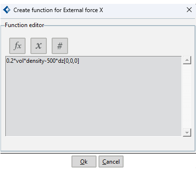
../../../_images/function_editor_interface.png — Fig. 1.96 Function editor interface.

A description of the operators can be used in the definition of functions are described.

Basic operators:

Table 1.5 Basic operators
Symbol	Description	Syntax
$+$	Adding operator.	`[adding_expression] + [adding_expression]`
$-$	Substraction operator.	`[subtraction_expression]-[subrtaction_expression]`
^	Exponent operator.	`[exponent_expression] ^ [function_expression]`
$*$	Multiplicative operator	`[multiplicative_expression] * [multiplicative_expression]`
/	Division operator.	`[multiplicative_expression] / [quotient_expression]`
$div$	Integer division operator $int(x/y+0.5)$	`([multiplicative_expression]) div ([quotient_expression])`. Example: (x)div(2+y)
$idiv$	Integer division operator $int(x/y+0.5)$. Similar to $div$. but with different syntax.	`([multiplicative_expression], [quotient_expression])`. Example: idiv(x,2+y)
$mod$	Integer division module operator $int(x+0.5)%int(y+0.5)$.	`([multiplicative_expression]) mod ([quotient_expression])`. Example: (t)mod(2).
$imod$	Integer division module operator int(x+0.5)%int(y+0.5). Similar to mod operator but with different syntax.	`imod ([multiplicative_expression],[quotient_expression])`. Example: imod(t,2).
$rdiv$	Real division operator int(x/y).	`([multiplicative_expression]) rdiv ([quotient_expression])`. Example: (t)rdiv(5).
$ddiv$	Real division operator int(x/y). Similar to rdiv operator but with different syntax.	`ddiv ([multiplicative_expression], [quotient_expression])`. Example: ddiv(t,5).
$rmod$	Real division module operator x/y-int(x/y).	`([multiplicative_expression]) rmod([quotient_expres-sion])`. Example: (t)rmod(5).
$dmod$	Real division module operator x/y-int(x/y). Similar to rmod operator but with different syntax.	`dmod ([multiplicative_expression],[quotient_expres-sion])` Example: dmod(t,5).
$max$	Maximum operator.	`max ([expression], [expression])`. Example: max(x,y)
$min$	Minimum operator.	`min ([expression], [expression])`. Example: min(x,y)
not	Not operator.	`not([function_expression])`
~	Not operator.	`~([function_expression])`

Examples:

$(2*dy)$
$(5*(dy+1))/2$
$(dz*dy)mod(5)$
$imod(dz*dy) (5)$
(5^4)

Relational operators:

The relational (binary) operators compare their first operand with their second operand to test validity of the specified relationship. The result of the relational expression is 1 if the tested relationship is true and 0 if it is false. The binary operators that can be used for functions definitions are:

Table 1.6 Relational operators
Symbol	Description	Syntax
$<$	Less than.	`[expression] < [expression]`
$<=$	Less or equal than.	`[expression]<[expression]`
$>$	Greater than.	`[expression] > [expression]`
$>=$	Greater or equal than.	`[expression]>[expression]`
$=$	Equal operator.	`[expression]=[expression]`
$!=$	Not equal operator.	`[expression]!=[expression]`
& or $\|$	And operator.	`[expression] & [expression]`

Examples:

$(dy>2)$
$(dx<=)$
$(dx!=1)$
$(dy>2)$ & $(dx>2)$

if-else statments:

The if statement controls conditional branching. The body of the if statement (elif_expression) is executed if the value of the expression is non zero. The syntax for the if statement is the following:

if (expression)then(elif_expression)else(next_expression)endif

being elif_expression an additional expression that may include an elif clause with next form:

(expression2)elif(elif_expression2)then(next_expression2)

Examples:

if(dy>2)then(if(x<1)then(1)else(0)endif)else(0)endif
if(dy>2)then(1)elif(dx<1)then(2)else(0)endif

Function operators:

The function operators calculate the value of a standard function at the point defined by the given argument. The function operators that can be used for the definition of the functions are:

Table 1.7 Function Reference
Function	Description	Syntax
sqrt	Calculates the square root of the argument.	`sqrt(.)`
abs	Calculates the absolute value of the argument.	`abs(.)`
ln	Logarithm of the argument, base e.	`ln(.)`
log	Logarithm of the argument, decimal base.	`log(.)`
fac	Factorial of the argument.	`fac(.)`
sin	Sine of the argument (given in radians).	`sin(.)`
cos	Cosine of the argument (given in radians).	`cos(.)`
tan	Tangent of the argument (given in radians).	`tan(.)`
asin	Arcsine of the argument in the range -π/2 to π/2 radians.	`asin(.)`
acos	Arccosine of the argument in the range 0 to À radians.	`acos(.)`
atan	Arctangent of the argument in the range -π/2 to π/2 radians.	`atan(.)`
sinh	Hyperbolic sine of the argument.	`sinh(.)`
cosh	Hyperbolic cosine of the argument.	`cosh(.)`
tanh	Hyperbolic tangent of the argument.	`tanh(.)`
exp	Calculates the exponential value of the argument.	`exp(.)`
heaviside	Evaluates the Heaviside function.	`heaviside(., .)`
interpolate	Performs linear interpolation based on given data.	`interpolate(#ξ1,η1,ξ2,η2,ξ3,η3,...#)`
interpolatespline	Performs spline interpolation based on given data.	`interpolatespline(#ξ1,η1,ξ2,η2,ξ3,η3,...#)`
InterpolateFile	Performs spline interpolation based on data from a file.	`InterpolateFile(., .)`
srand	Returns a pseudorandom integer in the range 0 to 1.	`srand(.)`
int	Integer conversion.	`int(.)`
(change sign operator)	Changes the sign of the expression.	`(-expression)`
j0	Calculates Bessel function of first kind and order 0.	`j0(.)`
j1	Calculates Bessel function of first kind and order 1.	`j1(.)`
jn	Calculates Bessel function of first kind and order n.	`jn(., .)`
y0	Calculates Bessel function of second kind and order 0.	`y0(.)`
y1	Calculates Bessel function of second kind and order 1.	`y1(.)`
yn	Calculates Bessel function of second kind and order n.	`yn(., .)`
Readfile	Executes the function in the ASCII file defined by the argument.	`readfile(.)`
Tcl	Executes a TCL script or procedure returning a double value.	`tcl(.)`
CloudOfDataFile	Performs local interpolation based on a cloud of points and data given in a file.	`CloudOfDataFile(.)`

Examples:

2 * sqrt(dy)
dx * fac(5)
srand(0)
log(abs(dx))
exp(5)
interpolate(#1.0,2.0,2.0,2.5,3.0,2.0#t^2)

Specific variables:

Furthermore, the following variables can be used in the definition of functions. Note that some of these variables refer to the main body (index 1). In order to access the corresponding variable for other bodies, the index of the body must be given in parentheses ( examples: dx(2)[0,0,0], vx(3) ).

1.4.7.1.1. General variables

Table 1.8 Parameters Reference
Parameter	Description	Units
time or t	Process time	s
gravity or g	Magnitude of gravity	m/s²
density	Fluid density	kg/m·s²
ts or dt	Time increment	s
Init_factor	Returns the current initialization factor (if the initialization time option is used)

1.4.7.1.2. Wave spectrum variables

Table 1.9 Wave Parameters Reference
Parameter	Description	Units
Hs	Significant wave height	m
Tm	Mean wave period	s
W_s	Wave frequency	s⁻¹
Gamma_s	Wave direction	º

1.4.7.1.3. Mesh general variables

These variables may be employed in the definition of boundary conditions varying in space thus resulting in functions that need to be evaluated at every boundary mesh node (for example to define the pressure distribution field within the pressurized free surface boundary condition).

x, y, z : coordinates of mesh points.

1.4.7.1.4. Free surface variables

Table 1.10 Node Parameters Reference
Parameter	Description	Units
eta[idNode]	Free surface elevation at the specified node
eta_prev[idNode]	Free surface elevation at the specified node (previous step)
x[idNode]	x coordinate at the specified node idNode
y[idNode]	y coordinate at the specified node idNode

1.4.7.1.5. Body’s variables

Table 1.11 Body Parameters Reference
Parameter	Description	Units
vol(idx) or volume(idx)	Water volume displaced by body idx	m³
disp	Mass of water displaced by body	kg
Wet_surface	Area of body surface under still water level	m²
xc(idx)	X coordinate of the buoyancy center of body idx	m
yc(idx)	Y coordinate of the buoyancy center of body idx	m
zc(idx)	Z coordinate of the buoyancy center of body idx	m
xg(idx)	X coordinate of the buoyancy center of body idx	m
yg(idx)	Y coordinate of the buoyancy center of body idx	m
zg(idx)	Z coordinate of the buoyancy center of body idx	m
k11(idx)	Surge hydrostatic restoring coefficient of body idx	N/m
k22(idx)	Sway hydrostatic restoring coefficient of body idx	N/m
k33(idx)	Heave hydrostatic restoring coefficient of body idx	N/m
k44(idx)	Roll hydrostatic restoring coefficient of body idx	N/rad
k55(idx)	Pitch hydrostatic restoring coefficient of body idx	N/rad
k66(idx)	Yaw hydrostatic restoring coefficient of body idx	N/rad
mass(idx)	Mass of body idx	kg
Ixx(idx)	Inertial moment of body idx with respect to X direction and gravity center	Kg·m²
Iyy(idx)	Inertial moment of body idx with respect to Y direction and gravity center	Kg·m²
Izz(idx)	Inertial moment of body idx with respect to Z direction and gravity center	Kg·m²
dx	Translation in the x direction of the main body gravity center	m
dy	Translation in the y direction of the main body gravity center	m
dz	Translation in the z direction of the main body gravity center	m
dx(bodyIdx,stepIdx)	Returns the translation along the x direction of the body given by bodyIdx at a previous time step given by stepIdx	m
dy(bodyIdx,stepIdx)	Returns the translation along the y direction of the body given by bodyIdx at a previous time step given by stepIdx	m
dz(bodyIdx,stepIdx)	Returns the translation along the z direction of the body given by bodyIdx at a previous time step given by stepIdx	m
dx[xi, yi, zi]	Translation in the x direction of an arbitrary point with coordinates [xi, yi, zi] with respect to the gravity center	m
dy[xi, yi, zi]	Translation in the y direction of an arbitrary point with coordinates [xi, yi, zi] with respect to the gravity center	m
dz[xi, yi, zi]	Translation in the z direction of an arbitrary point with coordinates [xi, yi, zi] with respect to the gravity center	m
ldsx	Translation in the x direction in the local frame	m
ldsy	Translation in the y direction in the local frame	m
ldsz	Translation in the z direction in the local frame	m
rx	Rotation around the x direction of the body gravity center	rad
ry	Rotation around the y direction of the body gravity center	rad
rz	Rotation around the z direction of the body gravity center	rad
rx(bodyIdx,stepIdx)	Returns the rotation around the x direction of the body given by bodyIdx at a previous time step given by stepIdx	rad
ry(bodyIdx,stepIdx)	Returns the rotation around the y direction of the body given by bodyIdx at a previous time step given by stepIdx	rad
rz(bodyIdx,stepIdx)	Returns the rotation around the z direction of the body given by bodyIdx at a previous time step given by stepIdx	rad
lrx	Rotation around the x direction in the local frame	rad
lry	Rotation around the y direction in the local frame	rad
lrz	Rotation around the z direction in the local frame	rad
vx	Body velocity in the x direction	m/s
vy	Body velocity in the y direction	m/s
vz	Body velocity in the z direction	m/s
vx(bodyIdx,stepIdx)	Returns the velocity in the x direction of the body given by bodyIdx at a previous time step given by stepIdx	m/s
vy(bodyIdx,stepIdx)	Returns the velocity in the y direction of the body given by bodyIdx at a previous time step given by stepIdx	m/s
vz(bodyIdx,stepIdx)	Returns the velocity in the z direction of the body given by bodyIdx at a previous time step given by stepIdx	m/s
wx	Body angular velocity around the x direction	rad/s
wy	Body angular velocity around the y direction	rad/s
wz	Body angular velocity around the z direction	rad/s
wx(bodyIdx,stepIdx)	Returns the angular velocity around the x direction of the body given by bodyIdx at a previous time step given by stepIdx	rad/s
wy(bodyIdx,stepIdx)	Returns the angular velocity around the y direction of the body given by bodyIdx at a previous time step given by stepIdx	rad/s
wz(bodyIdx,stepIdx)	Returns the angular velocity around the z direction of the body given by bodyIdx at a previous time step given by stepIdx	rad/s
lvx	Body velocity in the x direction in the local frame	m/s
lvy	Body velocity in the y direction in the local frame	m/s
lvz	Body velocity in the z direction in the local frame	m/s
lwx	Body angular velocity around the x direction in the local frame	rad/s
lwy	Body angular velocity around the y direction in the local frame	rad/s
lwz	Body angular velocity around the z direction in the local frame	rad/s
ax	Body acceleration in the x direction	m/s²
ay	Body acceleration in the y direction	m/s²
az	Body acceleration in the z direction	m/s²
ax(bodyIdx,stepIdx)	Returns the acceleration in the x direction of the body given by bodyIdx at a previous time step given by stepIdx	m/s²
ay(bodyIdx,stepIdx)	Returns the acceleration in the y direction of the body given by bodyIdx at a previous time step given by stepIdx	m/s²
az(bodyIdx,stepIdx)	Returns the acceleration in the z direction of the body given by bodyIdx at a previous time step given by stepIdx	m/s²
lax	Body acceleration in the x direction in the local frame	m/s²
lay	Body acceleration in the y direction in the local frame	m/s²
laz	Body acceleration in the z direction in the local frame	m/s²
arx	Body angular acceleration around the x direction	rad/s²
ary	Body angular acceleration around the y direction	rad/s²
arz	Body angular acceleration around the z direction	rad/s²
arx(bodyIdx,stepIdx)	Returns the angular acceleration around the x direction of the body given by bodyIdx at a previous time step given by stepIdx	rad/s²
ary(bodyIdx,stepIdx)	Returns the angular acceleration around the y direction of the body given by bodyIdx at a previous time step given by stepIdx	rad/s²
arz(bodyIdx,stepIdx)	Returns the angular acceleration around the z direction of the body given by bodyIdx at a previous time step given by stepIdx	rad/s²
larx	Body angular acceleration around the x direction in the local frame	rad/s²
lary	Body angular acceleration around the y direction in the local frame	rad/s²
larz	Body angular acceleration around the z direction in the local frame	rad/s²
HPFx_body	X component of the force due to hydrostatic pressure over the body	N
HPFy_body	Y component of the force due to hydrostatic pressure over the body	N
HPFz_body	Z component of the force due to hydrostatic pressure over the body	N
HPMx_body	X component of the moment due to hydrostatic pressure over the body	N·m
HPMy_body	Y component of the moment due to hydrostatic pressure over the body	N·m
HPMz_body	Z component of the moment due to hydrostatic pressure over the body	N·m
PFx_body	X component of the force due to dynamic pressure over body	N
PFy_body	Y component of the force due to dynamic pressure over body	N
PFz_body	Z component of the force due to dynamic pressure over body	N
PMx_body	X component of the moment due to dynamic pressure over body	N·m
PMy_body	Y component of the moment due to dynamic pressure over body	N·m
PMz_body	Z component of the moment due to dynamic pressure over body	N·m
TFx_body	X component of the total force over body	N
TFy_body	Y component of the total force over body	N
TFz_body	Z component of the total force over body	N
TMx_body	X component of the total moment over body	N·m
TMy_body	Y component of the total moment over body	N·m
TMz_body	Z component of the total moment over body	N·m
Fx_drift	X component of the drift load due up to first-order terms over body	N
Fy_drift	Y component of the drift load due up to first-order terms over body	N
Fz_drift	Z component of the drift load due up to first-order terms over body	N
Mx_drift	X component of the drift moment due up to first-order terms over body	N·m
My_drift	Y component of the drift moment due up to first-order terms over body	N·m
Mz_drift	Z component of the drift moment due up to first-order terms over body	N·m
Fx_Pdrift	X component of the drift load due up to first-order terms over body	N
Fy_Pdrift	Y component of the drift load due up to first-order terms over body	N
Fz_Pdrift	Z component of the drift load due up to first-order terms over body	N
Mx_Pdrift	X component of the drift moment due up to first-order terms over body	N·m
My_Pdrift	Y component of the drift moment due up to first-order terms over body	N·m
Mz_Pdrift	Z component of the drift moment due up to first-order terms over body	N·m
RFx_body	X component of the reaction loads over body	N
RFy_body	Y component of the reaction loads over body	N
RFz_body	Z component of the reaction loads over body	N
RMx_body	X component of the reaction moments over body	N·m
RMy_body	Y component of the reaction moments over body	N·m
RMz_body	Z component of the reaction moments over body	N·m

Deprecated variables:

Table 1.12 Depracted variables
dx_prev	Return body’s displacement (previous step)	m
dy_prev	Return body’s displacement (previous step)	m
dz_prev	Return body’s displacement (previous step)	m
rx_prev	Rotation, around the x direction, of the body gravity center (previous step).	rad
ry_prev	Rotation, around the y direction, of the body gravity center (previous step).	rad
rz_prev	Rotation, around the z direction, of the body gravity center (previous step).	rad
vx_prev	Body velocity in the x direction (previous step).	m/s
vy_prev	Body velocity in the y direction (previous step).	m/s
vz_prev	Body velocity in the z direction (previous step).	m/s
wx_prev	Body angular velocity around the x direction (previous step).	rad/s
wy_prev	Body angular velocity around the y direction (previous step).	rad/s
wz_prev	Body angular velocity around the z direction (previous step).	rad/s
ax_prev	Body acceleration in the x direction (previous step).	m/s²
ay_prev	Body acceleration in the y direction (previous step).	m/s²
az_prev	Body acceleration in the z direction (previous step).	m/s²
arx_prev	Body angular acceleration around the x direction in the local frame (previous step).	rad/s²
ary_prev	Body angular acceleration around the y direction in the local frame (previous step).	rad/s²
arz_prev	Body angular acceleration around the z direction in the local frame (previous step).	rad/s²

PRESSURIZED FREE SURFACE VARIABLES

Table 1.13 Pressurized Free Surface Variables
Symbol	Description	Units
Flux	Vertical airflow displaced by pressurized free surfaces.	m³/s
Flux(Idx,stepIdx)	Returns the vertical airflow displaced by the pressurized free surfaces indicated by Idx at a previous time step indicated by stepIdx.	m³/s
areap	Area of pressurized free surface.	m²
areapxm	X component of the gravity center of the pressurized free surface.	m
areapym	Y component of the gravity center of the pressurized free surface.	m
Pave	Average pressure applied over pressurized free surface.	Pa
P	Total pressure applied over pressurized free surface.	Pa
P(Idx,stepIdx)	Returns the total pressure applied over the pressurized free surfaces indicated by Idx at a previous time step indicated by stepIdx.	Pa
vol_P	Volume occupied by the pressurized free surface elevation.	m³
vol_P(body,stepIdx)	Returns the volume occupied by the pressurized free surfaces indicated by Idx at a previous time step indicated by stepIdx.	m³
Fx_Pfs	X component of the force due to the pressure over the pressurized free surface.	N
Fy_Pfs	Y component of the force due to the pressure over the pressurized free surface.	N
Fz_Pfs	Z component of the force due to the pressure over the pressurized free surface.	N
Mx_Pfs	X component of the moment due to the pressure over the pressurized free surface.	N·m
My_Pfs	Y component of the moment due to the pressure over the pressurized free surface.	N·m
Mz_Pfs	Z component of the moment due to the pressure over the pressurized free surface.	N·m

Deprecated Variables

Table 1.14 Deprecated Variables
Symbol	Description	Units
Flux_prev	Vertical airflow displaced by pressurized free surfaces at the previous time step.	m³/s
P_prev	Total pressure applied over pressurized free surface at the previous time step.	Pa
vol_P_prev	Volume occupied by the pressurized free surface elevation at the previous time step.	m³

HEIGHT-LIMITED FREE SURFACE CONDITION VARIABLES

Table 1.15 Height-Limited Free Surface Condition Variables
Symbol	Description	Units
Fx_Hfs	X component of the force due to the pressure over the height-limited free surface.	N
Fy_Hfs	Y component of the force due to the pressure over the height-limited free surface.	N
Fz_Hfs	Z component of the force due to the pressure over the height-limited free surface.	N
Mx_Hfs	X component of the moment due to the pressure over the height-limited free surface.	N·m
My_Hfs	Y component of the moment due to the pressure over the height-limited free surface.	N·m
Mz_Hfs	Z component of the moment due to the pressure over the height-limited free surface.	N·m

1.4.7.2. Appendix B: Tcl extension

SeaFEM can be extended by using the Tcl scripting language. Tcl, or the “Tool Command Language”, is a very simple, opensource-licensed programming language. Tcl provides basic language features such as variables, procedures, and control, and it runs on almost any modern OS, such as Unix, MacOS and Windows computers. But the key feature of Tcl is its extensibility. You may find further information on Tcl at:

http://wiki.tcl.tk/969

SeaFEM distribution includes a basic installation of Tcl, that allows to efficiently implement new capabilities in SeaFEM. However full Tcl installation provides many tool-kits and libraries that can help in the implementation of above mentions SeaFEM extensions. The full Tcl version can be downloaded from:

http://www.activestate.com/activetcl/

Finally, Ramdebbuger software can be used for editing and debugging Tcl code. Ramdebugger is free to use and can be downloaded from:

http://www.compassis.com/ramdebugger

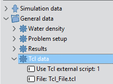
1.4.7.2.1. Initiating Tcl extension

SeaFEM Tcl extension is initiated by selecting the Tcl extension option available in the General data (Tcl data) page as shown in the following picture. If the check-box is selected, the Tcl extension of SeaFEM is activated. The entry must indicate a Tcl script to be interpreted during execution.

The Tcl script used for the SeaFEM extension can implement some standard SeaFEM Tcl event procedures (see TCL Interface procedures). These procedures are automatically called by SeaFEM during execution, when the Tcl interface is activated.

SeaFEM Tcl extension includes a basic library for vector operation and manipulation. Further information on the Tcl math library can be found in the Tdyn manual. The functions for vector manipulation can operate with temporal vector created from Tcl code and with internal SeaFEM variable vectors. Internal SeaFEM vectors can be accessed from the Tcl extension using standard names. A list of the SeaFEM vectors that can be accesses from the Tcl interface are provided next:

Symbol	Description
wxnd	Vector of x coordinates of the mesh nodes.
wynd	Vector of y coordinates of the mesh nodes.
wznd	Vector of z coordinates of the mesh nodes.
wph1	Vector of potential (Φ) nodal values (current value at t).
wphx	Vector of nodal values of the x derivatives of the potential (Φ).
wphy	Vector of nodal values of the y derivatives of the potential (Φ).
wphz	Vector of nodal values of the z derivatives of the potential (Φ).
wph2	Vector of potential (Φ) nodal values (previous value at tdt).
whfl	Vector of nodal values of the free surface elevation height limit.
whfp	Vector of nodal values of the pressure obtained due to free surface elevation height limit.

1.4.7.2.2. TCL Interface procedures

The Tcl script used for the SeaFEM extension can implement some of the following Tcl event procedures (as well as other user-defined procedures). These procedures (listed below) are automatically called by SeaFEM during execution, when the Tcl interface is activated. Their syntax corresponds to the standard Tcl language.

Function	Description
TdynTcl_InitiateProblem	Called at the beginning of the execution, after all data structures are created.
TdynTcl_FinishProblem	Called at the end of the execution of the current problem.
TdynTcl_StartSetProblem	Called before the creation of the main structures of the problem.
TdynTcl_EndSetProblem	Called once the creation of the main structures of the problem is finished.
TdynTcl_StartNewStep	Called when a new time step is started.
TdynTcl_FinishStep	Called when a time step is finished.
TdynTcl_StartNewIteration	Called when a new iteration is started.
TdynTclFinishIteration	Called when an iteration is finished.
TdynTcl_CreateBodyLinks	Called to initiate the body link conditions.
TdynTcl_DefineBodyData	Called to initiate the body link conditions, too.
TdynTcl_CreateMooring	Called to create mooring lines.
TdynTcl_InitiateHfs	Called within the algorithm of definition of the free surface height (HFreeSurface condition). Initiates the vector whfl.
TdynTcl_WriteResults time	Called after writing the results of the step. Argument gives the current time for writing the result data. Only called for specified time steps in the input data.
TdynTcl_StartTimeLoop	Called just before starting the time loop of the problem.
TdynTcl_Time	Returns the current simulation time.
TdynTcl_Dt	Returns the current time increment.
TdynTcl_Insert_Interpolator_Mesh interpolator_name initial/final mesh_id	Used to insert an internal SeaFEM mesh (mesh_id) in an interpolator structure (interpolator_name). The available meshes are: fluid, body, frees, outlet, inlet, pfrees and hfrees. See Examples of scripts defining a TCL extension for further information.
TdynTcl_Read_Interpolator_Mesh_ForHfs	Used to insert a mesh in GiD format (mesh_file) in an interpolator structure (interpolator_name) for imposing a free surface height condition.
TdynTcl_Create_Mooring_Segment	Used to create a mooring line. Arguments listed in the following.
TdynTcl_Read_Interpolator_Mesh_ForHfs interpolator_name initial/final mesh_file vector_id	This procedure can be used to insert a mesh in GiD format (mesh_file) in a interpolator structure (interpolator_name) for imposing a free surface height condition. See Examples of scripts defining a TCL extension for further information
TdynTcl_Create_Mooring_Segment body type xi yi zi xe ye ze w L A E [SN d1 d2]	This procedure can be used to create a mooring line. The different options to create mooring lines are presented in the section Appendix E: Mooring definition by Tcl. The arguments passed to this procedure are listed in what follows. Note that arguments within brackets only apply for certain types of mooring types (see argument’s description below)
TdynTcl_Create_Mooring_Link	This procedure creates a link between different mooring lines. The different options to create links are presented in the section Appendix E: Mooring definition by Tcl.
TdynTcl_Set_Mooring_Displacement seg1 fun1 fun2 fun3	This procedure can be used to specify the displacement of one end of the mooring line. The arguments are:
TdynTcl_Configure_Mooring_Segment Gk Gc Gu Cd Cf Cm alpha_bs gamma_bs bci steps	This procedure can be used to configure already existing mooring segments. It is only available for mooring segments of cable type. The arguments are:
TdynTcl_Configure_Mooring_Segment id load_curve [list e1 F1 e2 F2 … en Fn]	This procedure can be used to define a load-extension curve for a given dynamic cable. The arguments are:
TdynTcl_CreateBodyLinks	TdynTcl_CreateBodyLink can be used to create correlations between degrees of freedom from different bodies. This is internally implemented by using a Lagrange’s multipliers approach. This essentially consists on adding a matrix of restrictions to the bodies dynamics, each row of that matrix corresponding to the equation defining a link. The arguments passed to this function are triads of values that consecutively define the various coefficients of the link equation. To this aim, each triad consists on an integer identifying the body, another integer identifying the degree of freedom and a real value setting the corresponding coefficient value. An additional argument is given at he end to specify an optional independent coefficient that could exist for a given link equation. The different options to create body links are presented in the section Appendix D: Multi-body analysis.
TdynTcl_Give_Motions_For_Mesh body_id time mesh_file	This procedure calculates the displacements, velocities and acceleration of the nodes of a mesh mesh_file in GiD format) calculated from the motion data of the body body_id. The evaluation is done for time time. See Examples of scripts defining a TCL extension for further information TdynTcl_Add_Mass_Matrix body_id [list x y z] mass_matrix This procedure can be called first within the TdynTcl_InitiateProblem procedure to set the mass matrix of the body. The mass matrix must be a 6x6 matrix (given as a list of 36 elements) containing the mass and inertia elements of the different degrees of freedom of the body (surge, sway, heave,roll, pitch and yaw) refered to a point given by the coordinates (x ,y,z) that are also passed as a list argument to the procedure. This procedure overwrites the definition of mass and inertia inserted in the user interface. This procedure can be called within TdynTcl_StartNewStep to update the mass matrix of the body from that time step. In that case, the procedure TdynTcl_Build_Mass_Matrixes must be called afterwards. The arguments are:
TdynTcl_Add_Damping_Matrix body_id [list x y z] damping_matrix	This procedure can be called first within the TdynTcl_InitiateProblem procedure to set the damping matrix of the body. The damping matrix must be a 6x6 matrix (given as a list of 36 elements) containing the damping terms corresponding to the different degrees of freedom of the body (surge, sway, heave, roll, pitch and yaw) refered to a point given by the coordinates (x,y,z) that are also passed as a list argument to the procedure. This procedure can be called within TdynTcl_StartNewStep to update the damping matrix of the body from that time step. The arguments are:
TdynTcl_Add_Stiffness_Matrix body_id [list x y z] stiffness_matrix	This procedure can be called first within the TdynTcl_InitiateProblem procedure to set the stiffness matrix of the body. The stiffness matrix must be a 6x6 matrix (given as a list of 36 elements) containing the stiffness terms corresponding to the different degrees of freedom of the body (surge, sway, heave, roll, pitch and yaw) refered to a point given by the coordinates (x,y,z) that are also passed as a list argument to the procedure. This procedure can be called within TdynTcl_StartNewStep to update the stiffness matrix of the body from that time step. The arguments are:
TdynTcl_Give_Pressure_For_Mesh body_id time mesh_File	This procedure can be called to get the total pressure over the surface of a given body. Such pressure data is returned in the form of a list of pressure values for every node of the mesh provided. These pressure values are calculated by interpolating from the mesh of the required body. The arguments are:
TdynTcl_Set_Pfreesurface_Pressure Idx press	This procedure can be called to specify the total pressure press to be applied over the free surface of the PFreeSurface condition identified by Idx. The arguments are:

1.4.7.2.2.1. Examples of scripts defining a TCL extension

The scripts below show examples of procedures defining a SeaFEM Tcl extension. In order to execute these procedures, they have to be saved to a file and the file has to be inserted in the Tcl data page of General Data.

Tcl script example 1: Write a notice in info file

The following procedure (TdynTcl_StartNewStep) is executed at the beginning of every time step. It just writes a message to the standard SeaFEM output (Calculate > View process info…).

proc TdynTcl_StartNewStep { } {

  # Reading SeaFEM internal time
  set t [TdynTcl_Time]
  # Writing a message in SeaFEM info window
  TdynTcl_Message "Executing TdynTcl_StartNewStep: time $t" notice
}

Tcl script example 2: Loading Tk package

The following script loads Tk package. Tk is Tcl a library, including basic elements for building a graphical user interface. Once this library is loaded, graphic elements can be created from the Tdyn Tcl interface. In this example, a text window is created and then every time step, the text “Step $Current_Step$” is printed in that window. In the following code, the full Tcl installation is assumed to be in the directory “C:Program FilesTcllib”. The full Tcl installation can be downloaded from http://www.activestate.com/activetcl/.

# Define directory of the Tcl installation
lappend ::auto_path {C:\Program Files\Tcl\lib}
TdynTcl_Message [package require Tk] notice
# Creates a text window
pack [text .t -width 70 -height 20]
# Prints information in the text window
proc TdynTcl_StartNewStep { } {
  set time [TdynTcl_Time]
  .t ins end "Time $time\n" ; .t see end ; update
}

Tcl script example 3: Initiate Hfs

The following script initiates the free surface height of a surface (with HFreeSurface condition applied) by interpolating the z coordinate from a mesh file in GiD format (mesh.msh).

proc TdynTcl_InitiateHfs {} {
  # Initiate elevation
  TdynTcl_Message "Initiate z!!!" notice
  set inter2 [TdynTcl_Create_Interpolator]
  set tmpvec [::mather::mkvector 1 0.0]
  TdynTcl_Insert_Interpolator_Mesh $inter2 initial hfrees
  TdynTcl_Read_Interpolator_Mesh_ForHfs $inter2 final "mesh.msh" $tmpvec
  TdynTcl_OnInitial_Interpolator $inter2 $tmpvec whfl
  TdynTcl_Release_Interpolator $inter2
  vmdelete $tmpvec
}

Tcl script example 4: Communicate SeaFEM with Ramseries using HFreeSurface condition

The following script communicates in calculation time SeaFEM with Ramseries. SeaFEM sends to Ramseries (every time step) the pressure calculated on a HFreeSurface condition. Ramseries uses this information to apply a pressure load on the structure and send back the displacements of the structure, used in SeaFEM to update HFreeSurface condition (height elevation).

proc TdynTcl_InitiateHfs {} {
  # Initiate elevation
  TdynTcl_Message "Initiate z!!!" notice
  set inter2 [TdynTcl_Create_Interpolator]
  set tmpvec [::mather::mkvector 1 0.0]
  TdynTcl_Insert_Interpolator_Mesh $inter2 initial hfrees
  TdynTcl_Read_Interpolator_Mesh_ForHfs $inter2 final "mesh.msh"
  $tmpvec
  TdynTcl_OnInitial_Interpolator $inter2 $tmpvec whfl
  TdynTcl_Release_Interpolator $inter2
  vmdelete $tmpvec
}
proc TdynTcl_InitiateProblem {} {
  global myvec myvec2 myvec3 myrec nnode inter
  # nnRam must be set to the number of nodes of the structural mesh
  (fingers.msh)
  set nnRam 2619
  # Create the vectors
  set myvec [::mather::mkvector $nnRam 0.0]
  set myrec [::mather::mkvector $nnRam 0.0]
  set myvec2 [::mather::mkvector $nnRam 0.0]
  set myvec3 ""
  # Init coupling
  mather_initcoupling 0 2010 100000
  TdynTcl_Message "Connected!!!" notice
  # Insert mesh for interpolation (mesh.msh is the structural mesh)
  mather_insertcouplingmesh "mesh.msh"
  # Init interpolator structure to pass information from the updated HFs mesh to fingers.msh
  set inter [TdynTcl_Create_Interpolator]
  TdynTcl_Insert_Interpolator_Mesh $inter initial hfrees
  TdynTcl_Read_Interpolator_Mesh $inter final "mesh.msh"
}
proc TdynTcl_StartNewStep {} {
  global myvec myvec2 myvec3 myrec nnode inter
  set step [TdynTcl_Time]
  TdynTcl_Message "-------> Interpolate data of pressure to the
  structural mesh" notice
  TdynTcl_OnFinal_Interpolator $inter whfp $myvec
  TdynTcl_Message "-------> Starts to send pressure vector for time
  $step" notice
  # Note: Only first component (pressure) of the traction vector is sent
  mather_sendcouplingvector $myvec 0 $step
  TdynTcl_Message "-------> Vector sent for time $step" notice
}
proc TdynTcl_FinishStep {} {
  # return
  global myvec myvec2 myvec3 myvec4 myrec nnode inter
  set step [TdynTcl_Time]
  TdynTcl_Message "-------> Starts to retrieve displacement increment
  for time $step" notice
  # Only z component is used
  set data [mather_retrievecouplingheader]
  mather_retrievecouplingvector $myrec 0 $step
  set data [mather_retrievecouplingheader]
  mather_retrievecouplingvector $myrec 0 $step
  set data [mather_retrievecouplingheader]
  mather_retrievecouplingvector $myrec 0 $step
  TdynTcl_Message "-------> Info received for time $step" notice
  # Convergence check
  mather_sendcouplingconvergence $step 1
  set conv [mather_retrievecouplingconvergence]
  TdynTcl_Message "-------> Convergence check for time $step: $conv"
  notice
  # Interpolate and update the displacement
  if { $myvec3 eq "" } {
    set myvec3 [::mather::mkvector [::mather::vector_info length whfl]
    0.0]
    set myvec4 [::mather::mkvector [::mather::vector_info length whfl]
    0.0]
  }
  TdynTcl_OnInitial_Interpolator $inter $myrec $myvec3
  vmexpr whfl += $myvec3
  TdynTcl_Message "-------> TdynTcl_FinishStep" notice
}

Tcl script example 5: Debugging a Tcl script with Ramdebugger

RamDebugger is a graphical debugger for Tcl-TK. With RamDebugger, it is possible to make Local Debugging, where the debugger starts the program to be debugged. and Remote debugging, where the program to debug is already started and RamDebugger connects to it. The latter option will be used in this case.

Note

Remark: In Windows, it is necessary to load the package comm (not the standard, but the one modified in RamDebugger), in order to debug the program remotely.

To debug the following example:

Open it with Ramdebugger and set a breakpoint in the line “TdynTcl_Message “Set a breakpoint in this line” notice”.
Then execute Tdyn, and wait for a few seconds, until the execution freezes.
Go to Ramdebugger and select:

File > Debug on > Tdyn

Tdyn execution will restant until the breakpoint is found.

Note

Remark: If Tdyn is not included in the list of “Remote TCL debugging” programs, update the list by selecting:

File > Debug on > Update remotes

# Load package commR
# Change the directory below with the one where Ramdebugger is
intalled
lappend ::auto_path {C:/Utils/RamDebugger7.0/addons}
TdynTcl_Message [package require commR] notice
# This register Tdyn for debugging
comm::register Tdyn 1
# Add breakpoint beyond this point.
# breakpoints only work inside a proc.
proc TdynTcl_FinishStep {} {
TdynTcl_Message "Set a breakpoint in this line" notice
TdynTcl_Message "Click the arrow button to go to this line"
notice
}
# Program gets stopped here waiting for the debugger to connect
commR::wait_for_debugger

Tcl script example 6: Calculating rigid body motions for a mesh

The following script calculates rigid body displacements, velocities and accelerations for the nodes of a given mesh (GiD ASCII format) and writes the results in an ASCII file (GiD format).

proc TdynTcl_InitiateProblem { } {
  global resfile mshfile
  set mshfile "C:/Users/julio/Desktop/Current/spar_mesh.msh"
  set resfile "C:/Temp/spar_acc.res"
  set fileid [open $resfile w+]
  puts $fileid "GiD Post Results File 1.0"
  close $fileid
}

proc TdynTcl_WriteResults { time } {
  global resfile mshfile
  # Arguments for TdynTcl_Give_Motions_For_Mesh are body_index,
  time and mesh_file_name
  set acclist [TdynTcl_Give_Motions_For_Mesh 1 $time $mshfile]
  set fileid [open $resfile a]
  puts $fileid "Result \"Displacement (m)\" Body $time Vector
  OnNodes"
  puts $fileid "Values"
  set i 1
  foreach inode $acclist {
    puts $fileid "$i [lrange $inode 0 2]"
    incr i
  }
  puts $fileid "End Values"
  puts $fileid "Result \"Velocity (m/s)\" Body $time Vector OnNodes"
  puts $fileid "Values"
  set i 1
  foreach inode $acclist {
    puts $fileid "$i [lrange $inode 3 5]"
    incr i
  }
  puts $fileid "End Values"
  puts $fileid "Result \"Acceleration (m/s2)\" Body $time Vector
  OnNodes"
  puts $fileid "Values"
  set i 1
  foreach inode $acclist {
    puts $fileid "$i [lrange $inode 6 8]"
    incr i
  }
  puts $fileid "End Values"
  close $fileid
}

Tcl script example 7: Create mooring lines

The following script creates 3 quasi-static catenary mooring lines set at 120º to each other.

proc TdynTcl_CreateMooring { } {
  # Mooring line 1: type 2: catenary
  # arguments: body type xi[m] yi[m] zi[m] xe[m] ye[m] ze[m] w[N/m]
  L[m] A[m2] E[Pa]
  set cat1 [TdynTcl_Create_Mooring_Segment 1 2 -380.0 0.0 -210.0
  -4.15 0.0 -60.0 1350 -1 0.02 2.05e11]
  # Mooring line 2: type 2: catenary
  # arguments: type xi[m] yi[m] zi[m] xe[m] ye[m] ze[m] w[N/m] L[m]
  A[m2] E[Pa]
  set cat2 [TdynTcl_Create_Mooring_Segment 1 2 190.0 329.1 -210.0
  2.1 3.6 -60.0 1350 -1 0.02 2.05e11]
  # Mooring line 3: type 2: catenary
  # arguments: type xi[m] yi[m] zi[m] xe[m] ye[m] ze[m] w[N/m] L[m]
  A[m2] E[Pa]
  set cat3 [TdynTcl_Create_Mooring_Segment 1 2 190.0 -329.1 -210.0
  2.1 -3.6 -60.0 1350 -1 0.02 2.05e11]
  TdynTcl_Message "TdynTcl_CreateMooring finished!!!" notice
}

The following script creates a multi-segment delta line:

proc TdynTcl_CreateMooring { } {
  set type 3
  set area 1.13E-006
  set w 0.076
  set E 2.10E+011
  # segments
  set segA [create_mooring_segment $type -3.58 0.00 -2.07 -4.49 0.0
  -4.78 $w 2.9370 $area $E 0]
  set segB [create_mooring_segment $type -1.28 0.00 -1.89 -3.58 0.0
  -2.07 $w 2.5590 $area $E 0]
  set segC [create_mooring_segment $type -0.17 0.00 -0.64 -1.28 0.0
  -1.89 $w 1.7620 $area $E 0]
  set segD [create_mooring_segment $type -0.32 0.00 -2.99 -1.28 0.0
  -1.89 $w 1.5590 $area $E 0]
  # links
  create_mooring_link $segB $segA 230.0
  create_mooring_link $segC $segB $segD 0.0
}

The following script creates eight pre-stressed spring lines:

proc TdynTcl_CreateMooring { } {
  # Mooring lines: type 1: spring
  # arguments: body type xi[m] yi[m] zi[m] xe[m] ye[m] ze[m] w[N/m]
  L[m] A[m2] E[Pa]
  set cat1 [TdynTcl_Create_Mooring_Line 1 1 -26.0 -2.6 -150.0 -26.0
  -2.6 -47.0 386.7 102.52 0.00503 2.05e11]
  set cat2 [TdynTcl_Create_Mooring_Line 1 1 -26.0 2.6 -150.0 -26.0 2.6
  -47.0 386.7 102.52 0.00503 2.05e11]
  set cat3 [TdynTcl_Create_Mooring_Line 1 1 26.0 -2.6 -150.0 26.0 -2.6
  -47.0 386.7 102.52 0.00503 2.05e11]
  set cat4 [TdynTcl_Create_Mooring_Line 1 1 26.0 2.6 -150.0 26.0 2.6
  -47.0 386.7 102.52 0.00503 2.05e11]
  set cat5 [TdynTcl_Create_Mooring_Line 1 1 -2.6 26.0 -150.0 -2.6 26.0
  -47.0 386.7 102.52 0.00503 2.05e11]
  set cat6 [TdynTcl_Create_Mooring_Line 1 1 2.6 26.0 -150.0 2.6 26.0
  -47.0 386.7 102.52 0.00503 2.05e11]
  set cat7 [TdynTcl_Create_Mooring_Line 1 1 -2.6 -26.0 -150.0 -2.6
  -26.0 -47.0 386.7 102.52 0.00503 2.05e11]
  set cat8 [TdynTcl_Create_Mooring_Line 1 1 2.6 -26.0 -150.0 2.6 -26.0
  -47.0 386.7 102.52 0.00503 2.05e11]
  TdynTcl_Message "TdynTcl_CreateMooring finished!!!" notice
}

The following script creates a mooring line (spring), defining the displacement of the end point by functions.

proc TdynTcl_CreateMooring { } {
  set seg1 [TdynTcl_Create_Mooring_Segment 1 1 0.0 0.0 0.0 100.0 0.0
  0.0 0.0 100.0 0.1 1.0e6]
  set fun1 [::mather::create_function waves "1.0*sin(0.5*t);"]
  set fun2 [::mather::create_function waves "0.0;"]
  set fun3 [::mather::create_function waves "0.0;"]
  TdynTcl_Set_Mooring_Displacement $seg1 $fun1 $fun2 $fun3
  TdynTcl_Message "TdynTcl_CreateMooringLine finished!!!" notice
}

Tcl script example 8: Creating functions

This script creates a function ‘0.9*density*volume;’ at the beginning of the execution. Then a procedure My_Mass is created to evaluate that function. The procedure can be accessed from SeaFEM function fields, by using ‘tcl(My_Mass)’.

proc TdynTcl_InitiateProblem { } {
  global myfunc
  set myfunc [::mather::create_function waves "0.9*density*volume;"]
}
proc My_Mass { } {
  global myfunc
  set ret [::mather::evaluate_function $myfunc]
  TdynTcl_Message "My_Mass = $ret" notice
  return $ret
}

Tcl script example 9: Creating a body link

In this example, a link is provided between the surge degree of freedom of body 1 (x_1) and the surge and pitch degrees of freedom (x_2 and ry_2) of body 2. In this equation coefficients concerning x_1 and x_2 are 1.0 and -1.0 respectively, while the coefficient concerning ry_2 is the z-distance between the gravity center of the two bodies being equal to 2.0. No independent term exists for this link.

proc TdynTcl_CreateBodyLinks { } {
  # x_1 - x_2 + (zg_2-zg_1)*ry_2 = 0
  set blnk2 [create_body_link 1 1 1.0 2 1 -1.0 2 5 +2.0 0.0]
  TdynTcl_Message "Body link 1 finished!!!" notice
}

Tcl script example 10: Interpolate to an external mesh the pressure acting on a given body

The following script interpolates into an external mesh representing a cylinder, the pressure acting on the main body of the simulation (body number 1). The operation is performed every time step and the results are written into a text file using GiD results format.

proc TdynTcl_InitiateProblem { } {
    global mshfile resfile
    set mshfile "Cylinder.msh"
    set resfile "Cylinder.flavia.res"
    set fileid [open $resfile w+]
    puts $fileid "GiD Post Results File 1.0"
    close $fileid
}

proc TdynTcl_FinishStep { } {
    global mshfile resfile
    set time [TdynTcl_Time]
    set acclist [TdynTcl_Give_Pressure_For_Mesh 1 $time $mshfile]
    set fileid [open $resfile a]
    puts $fileid "Result \"Pressure (Pa)\" Body $time Scalar OnNodes"
    puts $fileid "Values"
    set i 1
    foreach inode $acclist {
        puts $fileid [lrange $inode 0 1]
        incr i
    }
    puts $fileid "End Values"
    close $fileid
}

Tcl script example 11: Defining a mass matrix

The following script illustrates how to define the mass matrix of a body taking a generic point as the reference point for that matrix. Note that the mass matrix can be directly introduced within the graphic user interface of SeaFEM only in the case the matrix is known for the center of gravity. Hence, the tcl script procedure is useful when the mass matrix is known from a generic reference point that may differ from the center of gravity. If this is the case, the mass matrix in the graphic user interface is left empty, and the following tcl script is used to set up the mass matrix for the generic reference point. SeaFEM takes care of transforming the mass matrix from the reference point specified in the tcl script to the center of gravity or any other generic point specified for the sake of output in the user interface. In the present example, the generic point from which the mass matrix is specified is the point of coordinates (15, -25, -7). The first argument in the TdynTcl_Add_Mass_Matrix procedure indicates that the specified mass matrix concerns body number 1.

.. code-block:: tcl

  proc TdynTcl_InitiateProblem { } {
      TdynTcl_Add_Mass_Matrix 1 [list 15 -25 -7] [list
      1607.95 0 0 0 11255.65 -40198.75
      0 1607.95 0 -11255.65 0 -24119.25
      0 0 1607.95 40198.75 24119.25 0
      0 -11255.65 40198.75 1085366 602981 168835
      11255.65 0 24119.25 602981 442186.3 -281391.3
      -40198.75 -24119.25 0 168835 -281391.3 1368365 ]
      TdynTcl_Message "TdynTcl_InitiateProblem finished!!!" notice
  }

1.4.7.3. Appendix C: RAO analysis

When carrying out RAO analysis using the white noise spectrum, it must be taken into account that the SeaFEM RAO’s calculation is based on a discrete Fourier transform decomposition.

Because of this, the total calculation time and the sampling time are automatically calculated and fixed internally by the solver based on the maximum and the minimum frequencies (periods) specified by the user in the graphic user interface.

Hence, even if a “Simulation time” and/or a “Time step” are specified by the user, they will be ignored and fixed internally by SeaFEM. Only the “Initialization time” parameter will maintained since it can be useful to avoid energetic transient. This is because a sudden initialization (which can occur when no initialization time is specified) might lead to large accumulation of energy by the body, which would require longer simulation to dissipate all that unrealistic body energy.

1.4.7.4. Appendix D: Multi-body analysis

SeaFEM can perform analysis of multi-body configurations. In newer versions of SeaFEM, all bodies can be defined through the graphic user interface. To this aim, as many body data conditions as needed can be defined and assigned to the corresponding geometric entities. In the figure below for instance, two linked body data conditions were assigned to body1 and body2 groups that correspond to the 2 cylinders shown.

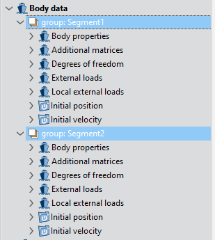
../../../_images/body_properties_2bodies.png

Hence, each group has assigned its own body properties, degrees of freedom, external loads and initial positions and velocities. Nevertheless, if any property within the condition is specified using a function, the variables used still require the body index to be indicated between parenthesis. For example, if body mass is defined using a function of the form $M = vol*density$ the actual body to which the variable vol applies must be indicated between parenthesis. Hence, the mass of the first body would actually read $M = vol(1)*density$ and so on. Keep in mind that body indices are assigned in the same order the bodies are defined in the data tree.

The results (movements, forces, etc.) of all bodies, are saved in the model folder, in the files ‘$model_name$.BodyKinematics.res’ and ‘$model_name$.BodyLoads.res’. Furthermore, they can be visualized in the ‘SeaFem graphs’ option of the Postprocess menu.

1.4.7.4.1. Body links

Within SeaFEM, it is also possible to define links between different bodies. This can be done in two ways.

First, action-reaction forces exerted between to given bodies can be introduced as external loads acting on the corresponding bodies. These functions use the standard syntax shown in section (Appendix A: function editor), but it is extended for multibodies analysis, by adding the index of the body between parenthesis at the end of the function. The following are some examples of this extension:

mass(2): mass of the body of index 2.
dx[1.0,1.0,1.0](1): displacement of the point 1.0,1.0,1.0 of the body of index 1.
yg(3): Y coordinate of the center of gravity of the body of index 3.

Secondly, links can also be created that correlate degrees of freedom from different bodies. This is internally implemented by using a Lagrange’s multipliers approach. This essentially consists on adding a matrix of restrictions to the bodies dynamics system, each row of that matrix corresponding to the equation defining a link. At the user’s level, it is necessary to define these kind of links by using a tcl script procedure. In particular, a Tcl procedure named TdynTcl_CreateBodyLinks must be reimplemented by the user in the tcl script. Within these procedure, several types of joints between bodies (each implying different number of body links) can be defined following the syntax detailed below. In addition, body links can be optionally updated at each iteration to take into account large displacements and rotations. To this aim, a Tcl procedure named TdynTcl_StartNewIteration must be reimplemented by the user in the tcl script. The syntax of the tcl functions used to update the joints (links) is identical to their creation counterpart just adding a first argument to identify the constraint equation index to be updated.

The type of body joints currently available within SeaFEM is listed bellow:

Rotation constraint

Line constraint

Plane constraint

Rotation link

Translation link

Rigid body joint

Ball joint

Revolute joint

Cylindrical joint

Prismatic joint

Translational joint

Next, the above body constraints and mechanical joints are described in detail alongside with the arguments required to define each one of the body link relations.

Rotation constraint

This type of constraint is used to prevent body rotation around an arbitrary given direction.
```
create_rotation_constraint #body #a #b #c

update_rotation_constraint #ilink #body #a #b #c
```
Argument #body1 must be an integer value (greater than 0) and is used to identify the body affected by the rotation constraint. Such an index must respond to the order of creation of the bodies in the interface. Arguments #a #b #c are the direction cosines of the axis about which the rotation of the body is prevented.
Line constraint

This type of constraint is used to enforce body movement along a given direction (the body is allowed to move only along a given direction).
```
create_line_constraint #body #a #b #c

update_line_constraint #ilink #body #a #b #c
```
Argument #body1 must be an integer value (greater than 0) and is used to identify the body affected by the line constraint. Such an index must respond to the order of creation of the bodies in the interface. Arguments #a #b #c are the direction cosines of the direction along which the body can move.
Plane constraint

This type of constraint is used to enforce body movement over a given plane. The body is allowed to move only over a plane whose normal is given and going through the initial position of the body’s reference point.
```
create_plane_constraint #body #a #b #c

update_plane_constraint #ilink #a #b #c
```
Argument #body1 must be an integer (greater than 0) and is used to identify the body to which the plane constraint applies.

This body index must be consistent with the order of creation of the bodies in the user interface. Arguments #a #b #c are the direction cosines of the plane’s normal direction.
Rotation constraint

This type of joint is used to enforce the rotation degree of freedom of two different bodies to be the same.
```
create_rotation_link #body1 #body2 #rotdof

update_rotation_link #ilink #body1 #body2 #rotdof
```
Arguments #body1 and #body2 must be integer values greater than 0 and are used to identify the two bodies being joined by the rotation link. These indexes correspond to the order of creation of the bodies in the interface. Argument #rotdof must be an integer value between 1 and 3 and is used to identify the constrained rotational degree of freedom (1 = Roll, 2 = Pitch, 3 = Yaw). Argument #ilink identifies the constraint equation index to be updated. It usually corresponds to an integer variable previously initialized by the return value of the create_link function.
Translation constraint

This type of link is used to create a constraint between translational degrees of freedom of 2 bodies.
```
create_translation_link #body1 #body2 #transdof

update_translation_link #ilink #body1 #body2 #transdof
```
Arguments #body1 and #body2 must be integer values (greater than 0) and are used to identify the two linked bodies. These indexes correspond to the order of creation the different bodies in the interface. Argument #transdof must be an integer value between 1 and 3 and is used to identify the constrained translational degree of freedom (1 = Surge, 2 = Sway, 3 = Heave). Argument #ilink identifies the constraint equation index to be updated. It usually corresponds to an integer variable previously initialized by the return value of the create_link function.
Rigid body joint

This type of joint can be used to enforce two different bodies to move as a single rigid body. The advantage of modelling the rigid body as two separate components instead of a unique body, is that forces and moments exerted by one component over the other are then accessible in the form of body joint reactions.
```
create_rigid_body_full_link #body1 #body2

update_rigid_body_full_link #ilink #body1 #body2
```
Arguments #body1 and #body2 must be integer values greater than 0 and are used to identify the two components of the rigid body set. These indices must correspond to the order the bodies were created in the user interface. Argument #ilink identifies the constraint equation index to be updated. It usually corresponds to an integer variable previously initialized by the return value of the create_link function.
Ball joint

This type of link is used to create a ball joint constraint between 2 bodies. This means that the two bodies being joined share a common point (usually the ball joint position point) about which both bodies can rotate freely.
```
create_ball_joint_link #body1 #body2 #x #y #z

update_ball_joint_link #ilink #body1 #body2 #x #y #z
```
Arguments #body1 and #body2 must be integer values greater than 0 and are used to identify the two linked bodies. These indexes correspond to the order of creation of the different bodies in the interface. Arguments #x, #y and #z must be real values that define the initial global position of the ball joint. Argument #ilink identifies the constraint equation index to be updated. It usually corresponds to an integer variable previously initialized by the return value of the create_link function.
Revolute joint

This type of joint is used to create a revolute constraint between 2 bodies. This type of junction implies that the two bodies can freely rotate about a common axis (actually the bodies share two points aligned on a given axis), while the remaining degrees of freedom (translation and rotation) are linked.
```
create_revolute_joint_link #body1 #body2 #x1 #y1 #z1 #x2 #y2 #z2
update_revolute_joint_link  #ilink #body1 #body2 #x1 #y1 #z1 #x2 #y2 #z2
```
Arguments #body1 and #body2 must be integer values greater than 0 and are used to identify the two bodies joined through the revolute joint. These indexes correspond to the order of creation of the different bodies in the interface. Arguments #x1, #y1, #z1 and #x2, #y2, #z2 must be real values defining the two points shared by the bodies. Actually these points define the common axis of revolution.
Cylindrical joint

This type of link is used to create a cylindrical joint between 2 bodies. A cylindrical joint implies that the two bodies can undergo relative translation along a given axis and relative rotation about the same axis. All the remaining degrees of freedom are linked.
```
create_cylindrical_joint_link #body1 #body2 #a #b #c
update_cylindrical_joint_link #ilink #body1 #body2 #a #b #c
```
Arguments #body1 and #body2 must be integer values greater than 0 and are used to identify the two bodies linked by the cylindrical joint. These indexes correspond to the order of creation of the different bodies in the interface. Arguments #a #b and #c must be real values that define the vector/axis that characterizes the cylindrical joint. Argument #ilink identifies the constraint equation index to be updated. It usually corresponds to an integer variable previously initialized by the return value of the create_link function.
Prismatic joint (deprecated)

This type of link is used to create a prismatic joint constraint between 2 bodies. A prismatic joint means that all rotational degrees of freedom are linked (this is, both bodies undergo identical roll, pitch and yaw rotations) and that both bodies can undergo relative translation only along a given axis. Such an axis is limited to be aligned along one of the global coordinate system axes (i.e. X, Y, or Z global axes). This type of link is deprecated and superseded by the Translational joint described below. Nevertheless, Prismatic joint are still available to ensure backward compatibility.
```
create_prismatic_joint_link #body1 #body2 #axis
update_prismatic_joint_link #ilink #body1 #body2 #axis
```
Arguments #body1 and #body2 must be integer values greater than 0 and are used to identify the two joined bodies. These indexes correspond to the order of creation the different bodies in the interface. Argument #axis must be an integer value greater than 1 that determines the axis along which the two bodies can undergo relative displacement. Argument #ilink identifies the constraint equation index to be updated. It usually corresponds to an integer variable previously initialized by the return value of the create_link function.
Translational joint

This type of link generalizes the prismatic joint. It is used to create a prismatic joint constraint between 2 bodies so that all rotational degrees of freedom are linked (this is, both bodies undergo identical roll, pitch and yaw rotations) while both bodies can undergo relative translation along a given generic axis.
```
create_prismatic_joint_link #body1 #body2 #a #b #c
update_prismatic_joint_link #ilink #body1 #body2 #a #b #c
```
Arguments #body1 and #body2 must be integer values greater than 0 and are used to identify the two joined bodies. These indexes correspond to the order of creation the different bodies in the interface. Arguments #a #b #c must be real values that define the vector/axis that characterizes the translational joint. Argument #ilink identifies the constraint equation index to be updated. It usually corresponds to an integer variable previously initialized by the return value of the create_link function.

Examples of tcl script with body joints

An example of tcl script procedure reads as follows:

proc TdynTcl_CreateBodyLinks { } {
  global link1 link2
  set link1 [create_ball_joint_link 1 2 0.0 0.0 -1.0]
  set link2 [create_rotation_link 1 2 0]
}

proc TdynTcl_StartNewIteration { } {
  global link1 link2
  update_ball_joint_link $link1 1 2 0.0 0.0 -1.0
  update_rotation_link $link2 1 2 0
}

In this example, first a ball joint link is created between bodies 1 and 2 (the corresponding equation index is stored in the global variable link1). The ball joint is located at the position given by the initial global coordinates 0.0, 0.0, -1.0. Secondly, an additional constraint between bodies 1 and 2 is created so that both bodies rigidly rotate in roll direction (link 2). Generic links can also be created that correlate any number of degrees of freedom from different bodies. The implementation of this kind of links essentially consists on calling the TdynTcl_Create_Body_Link function through the Tcl script. The arguments passed to this function are triads of values that consecutively define the various coefficients of the particular link equation. To this aim, each triad consists on an integer identifying the body, another integer identifying the degree of freedom and a real value setting the corresponding coefficient value. An additional argument can be provided at the end to specify an optional independent coefficient that could exist for a given link equation.

An example of tcl script procedure for this kind of generic link would read as follows:

proc TdynTcl_CreateBodyLinks { } {
  # x_1 - x_2 + (zg2 - zg1)*ry_2 = 0
  TdynTcl_Create_Body_Link 1 1 1.0 2 1 -1.0 2 5 2.0 0.0
}

In this example, a link is provided between the surge degree of freedom of body 1 and the surge degree of freedom of body 2. In this equation, coefficients concerning x_1 and x_2 are 1.0 and -1.0 respectively, while the coefficient concerning ry_2 is the z-distance between the gravity center of the two bodies (zg2 - zg1) being equal to 2.0. No independent term exists for this link. It is also possible to define links between bodies using the different mooring options of SeaFEM. See (Appendix E: Mooring definition by Tcl) section for further information.

1.4.7.5. Appendix E: Mooring definition by Tcl

Mooring definition in SeaFEM can be done by using the GUI options available (see Mooring data section for further information). However, mooring systems can also be defined through a Tcl script procedure, that gives access to advanced mooring definition options. The Tcl procedure must be implemented in a text file. Such a file, is further provided as an input argument of the Tcl data section of the data tree, once the option to use an external Tcl script is activated.

Tcl data can be accessed and modified at any time through the menu option:

General data > Tcl data

The procedure to be implemented in the tcl script is named TdynTcl_CreateMooringLine and simply consists on the definition of all mooring segments and further definition of the segment links. Segments definition is performed by calling the SeaFEM internal function create_mooring_segment. Arguments passed to this function are described below. Links between segments are specified by calling the SeaFEM internal function create_mooring_link. Arguments passed to this function are also described below.

The syntax to call TdynTcl_Create_Mooring_Segment and the arguments passed to the function are as follows:

TdynTcl_Create_Mooring_Segment $body $type $xi $yi $zi $xe $ye $ze $w $L $A $E [$S $N $d1 $d2]

Alternative syntax:

create_mooring_segment $body $type $xi $yi $zi $xe $ye $ze $w $L $A $E [$S $N $d1 $d2]

The arguments between brackets only apply to certain types of mooring segments.

body : index of the body to which the mooring is linked (from 1 to n). If unspecified, the current mooring segment is assumed to be attached to the main body.
type : determines the type of mooring segment to be used. Possible values:
- type = 4 - catenary
- type = 1 - spring
- type = 3 - spring only traction
- type = 6 - dynamic cable
xi [m] : x coordinate of the initial point of the mooring segment (closer to the body).
yi [m] : y coordinate of the initial point of the mooring segment (closer to the body).
zi [m] : z coordinate of the initial point of the mooring segment (closer to the body).
xe [m] : x coordinate of the end point of the mooring segment.
ye [m] : y coordinate of the end point of the mooring segment.
ze [m] : z coordinate of the end point of the mooring segment.
w [N/m] : effective weight (actual weight minus buoyancy) per unit length.
L [m] : length of the segment.
A [m^2] : cross-sectional area of the cable.
E [Pa] : Young modulus.
S : seabed parameter. This argument only affects catenary segments and dynamic cables. If provided for other mooring types, it will be ignored.
- S = 0 - No seabed contact. The segment has at both ends a ‘Connection point’, or a ‘Connection point’ and a ‘Fairlead point’.
- S = 1,..,7 - The segment has an ‘Anchor point’. Possible values:
  - S = 1 - Frictionless seabed (no seabed friction).
  - S = 2 - Chain with sandy seabed (chain + sandy seabed contact exist).
  - S = 3 - Chain with mud/sand seabed (chain + mud/sand seabed contact exist).
  - S = 4 - Chain with mud/clay seabed (chain + mud/clay seabed contact exist).
  - S = 5 - Wire rope with sandy seabed (wire rope + sandy seabed contact exist).
  - S = 6 - Wire rope with mud/sand seabed (wire rope + mud/sand seabed contact exist).
  - S = 7 - Wire rope with mud/clay seabed (wire rope + mud/clay seabed contact exist).
N : This argument only applies in the case of dynamic cables (type 6). It indicates the number of line elements for cable geometric discretization.
d1, d2 : User defined damping ratios.

For each segment, initial and end points must be introduced in a specific order, being the initial point the closest one to the body. The function simply returns an identifier for the created segment, that can be used to define links among the different mooring segments. These links are defined using the function create_mooring_link, as defined in the following. By default, create_mooring_segment assumes that the initial point is linked to the given body, and the end point is fixed at the seabed. However, this assumption can be overwritten by defining links with other mooring segments or bodies. As commented above, the function create_mooring_link can be used to define links among the different segments of a multisegment mooring line. This function can create different type of links as explained below.

The syntax to call create_mooring_link and the arguments passed to the function are as follows:

create_mooring_link $seg1 $seg2 $f

Alternative syntax:

TdynTcl_Create_Mooring_Link $seg1 $seg2 $f

Where:

seg1 : identifier variable corresponding to the first segment of the link (this must be the segment closer to the body).
seg2 : identifier variable corresponding to the second segment of the link.
f [N] : buoyancy force to be applied at the link node.

The operator TdynTcl_Create_Mooring_Link can also be used to define links between three lines (joint to the same node). In that case, the syntax of the function is as follows:

TdynTcl_Create_Mooring_Link $seg1 $seg2 $seg3 $f

Alternative syntax:

create_mooring_link $seg1 $seg2 $seg3 $f

seg1 : identifier variable corresponding to the first segment of the link (the segment closer to the body).
seg2 : identifier variable corresponding to the second segment of the link.
seg3 : identifier variable corresponding to the third segment of the link.
f [N] : buoyancy force to be applied at the link node.

The function TdynTcl_Create_Mooring_Link can also be used to define links between two bodies. In that case, the syntax of the function is as follows:

TdynTcl_Create_Mooring_Link $seg1 &body

Alternative syntax:

create_mooring_link $seg1 &body

seg1 : identifier variable corresponding to the segment of the link.
body : index of the body to which the mooring is linked (from 1 to n)

An example of a TCL script for defining a multi-catenary mooring system is shown below. It corresponds to the mooring system configuration sketched in the following figure:

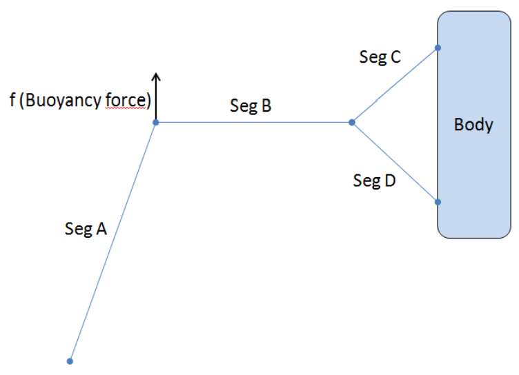
../../../_images/mooring_system_configuration_example.png — Fig. 1.98 Example of mooring system configuration.

proc TdynTcl_CreateMooring { } {
  set type 3
  set area 1.13E-006
  set w 0.076
  set E 2.10E+011
  # segments
  set segA [create_mooring_segment $type -3.58 0.00 -2.07 -4.49
  0.0 -4.78 $w 2.9370 $area $E 0]
  set segB [create_mooring_segment $type -1.28 0.00 -1.89 -3.58
  0.0 -2.07 $w 2.5590 $area $E 0]
  set segC [create_mooring_segment $type -0.17 0.00 -0.64 -1.28
  0.0 -1.89 $w 1.7620 $area $E 0]
  set segD [create_mooring_segment $type -0.32 0.00 -2.99 -1.28
  0.0 -1.89 $w 1.5590 $area $E 0]
  # links
  create_mooring_link $segB $segA 230.0
  create_mooring_link $segC $segB $segD 0.0
}

The function TdynTcl_Set_Mooring_Displacement can be used to define the displacement of the end point of a mooring segment.

Syntax:

TdynTcl_Set_Mooring_Displacement $seg1 $fun1 $fun2 $fun3

Alternative syntax:

set_mooring_displacement $seg1 $fun1 $fun2 $fun3

seg1 : identifier variable corresponding to the segment.
fun1 : index of the function describing the time-dependent displacement in OX of the end point of the mooring segment.
fun2 : index of the function describing the time-dependent displacement in OY of the end point of the mooring segment.
fun3 : index of the function describing the time-dependent displacement in OZ of the end point of the mooring segment.

The function TdynTcl_Configure_Mooring_Segment can be used to configure advanced options of the cable segments.

Syntax:

TdynTcl_Configure_Mooring_Segment $seg1 $Gk $Gc $Gu $Ms $Md $Cd $Cf $Cm $alpha $bci

Alternative syntax:

configure_moorin_segment $seg1 $Gk $Gc $Gu $Ms $Md $Cd $Cf $Cm $alpha $bci

where:

seg1 : identifier variable corresponding to the segment.

Gk : ground normal stiffness per unit length (Pa/m) for seabed interaction.

Gc : ratio of critical damping of ground (-) for seabed interaction.

Gu : horizontal damping coefficient (-) for seabed interaction.

Ms : static horizontal friction coefficient (-) for seabed interaction.

Md : dynamic horizontal friction coefficient (-) for seabed interaction.

Cd : tangential drag coefficient of the cable.

Cf : normal drag coefficient of the cable.

Cm : added mass coefficient of the cable.

alpha : Alpha coefficient of the Bossak-Newmark integration scheme.

bci : boundary condition for the initial node: 1 if acceleration is imposed, -1 if the node is fixed, 0 if it is free.

When running a SeaFEM analysis that includes mooring lines defintion, specific result files are generated concerning the mooring system:

MooringLoads.res - It contains the forces and moments exherted by the mooring system on the attached body.
MooringResults.msh - It contains an authomatically generated mesh of the mooring system.
MooringResults.res - It contains the displacement results of each mooring segment.
projectName.MooringData.res - It contains the tension force components at both ends of each mooring segment.

If MooringResults.msh and MooringResults.res files exist, they are authomatically loaded into the postprocessor graphic user interface. All mooring segments appear grouped within a single Mesh group called “Mooring”. Visualization options of each mooring segment can be manipulated individually as can be done with any other mesh. Mooring displacement results can also be animated by drawing the corresponding deformed result as shown in the figure below. To this aim, follow the steps listed in what follows:

In the meshes window, check all mooring segments that you want to be plotted.

Select the Mooring > Displacement > Contour fill option in the results window.

Choose the Deformed > Result > Mooring > {Displacement} option in the preferences window.

Finally, activate the Deformed > Draw option in the preferences window.

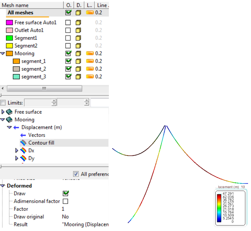
../../../_images/mooring_deformed_draw.png — Fig. 1.99 Drawing the corresponding deformed result.

1.4.7.6. Appendix F: Morison’s forces effect

When viscous effects may be advanced to have a significant effect on the dynamic behavior of an offshore structure, Morison’s equation can be used to correct the forces evaluated by the diffraction-radiation solver. For this purpose, an auxiliary framework structure, associated to a body must be defined. Based on the information provided by the user, SeaFEM evaluates Morison’s forces per unit length acting on this framework structure. After integration along the different elements, the resultant forces are incorporated to the dynamic solver of the rigid body to which the idealized framework structure has been associated.

To this aim, a tcl procedure must be used to define the different elements of the framework structure associated to a body. This procedure allows specifying the reference line of the element as well as the added mass, lift, drag and friction coefficients of the Morison’s equation. This function can be called several times to define as many elements as required.

The syntax to define the Tcl procedure to create new elements of the framework structure read as follows:

TdynTcl_Add_Morison_Element b t x1 y1 z1 x2 y2 z2 D S CM CD CV CF CL

where:

b is an integer index that identifies the body to which the Morison element pertains.

t is the element type (0 defines a standard element for which the floatability forces are evaluated, and 1 defines a virtual element for which floatability forces are neglected).

x1, y1, z1, x2, y2, z2 are the coordinates of the end points of the cylinder.

D is the section characteristic linear dimension (the diameter in the case of a cylinder).

S is the cross-sectional area.

CM is the added mass correction coefficient.

CD is the non-linear drag coefficient.

CV is the linear drag coefficient.

CF is the friction coefficient.

CL is the lift coefficient.

TdynTcl_Add_Morison_Element procedure returns the index of the created element of the framework structure.

Based on the information provided in the successive calls to TdynTcl_Add_Morison_Element command, SeaFEM evaluates Morison’s forces per unit length acting on the framework structure defined by the suer. After integration, the resultant forces are incorporated to the dynamics of the rigid body to which the framework structure has been associated. The various (per unit length) contributions to the force are calculated as follows:

$F_{M}=(1-\delta_{v})(1+C_{M}) \cdot \rho \cdot S \cdot (Ixa_{w}xI) - \rho \cdot S \cdot C_{M}(Ixa_{b}xI)$

$F_{D}=0.5 \cdot C_{D} \cdot \rho \cdot D |IxvxI| (IxvxI)$

$F_{V}=0.5 \cdot C_{V} \cdot \rho \cdot D (IxvxI)$

$F_{F}=0.5 \cdot C_{F} \cdot \rho \cdot \pi \cdot D |I \cdot v| (I \cdot v) \cdot I$

$F_{L}=0.5 \cdot C_{L} \cdot \rho \cdot D |Ixv| (Ixv)$

where

I is the unit vector locally oriented along the element,

a_wis the fluid acceleration of the incident wave,

a_bis the acceleration vector of any point of the body,

v is the relative velocity vector,

FM, FD, FV, FF and FL are the inertial correction, drag, linear drag, friction and lift components of the force per unit length respectively.

Note

Remarks: the first term in the right hand side of the F_Mequation includes the Froude-Kriloff force (i.e. the undisturbed wave pressure force) and the diffraction inertial force, while the second term represents the radiation inertial force.

It is important to keep in mind that the added mass contribution calculated using the Morison’s equation will be added to the added mass effect that is already accounted for by the diffraction-radiation SeaFEM solver. Hence, the added mass contribution of the Morison’s equation must be only used if, for some reason, the user wishes to correct the added mass effect calculated by SeaFEM.

It is emphasized that SeaFEM will always calculate the inertia term by integrating the pressure field on the body surface. This will result in the evaluation of the Froude-Krylov force plus diffraction force. On the other hand, it is well known that viscous effects can reduce the amplitude of the diffraction force, and in most of the cases SeaFEM calculation will result in overprediction of this value. Hence, the added mass contribution of the Morison’s equation can be used to improve the computational prediction of this force, by setting a suitable (usually negative) value of C_M, based on experimental information.

As an example, the following code can be used to add to body number 1 the Morison forces acting on a cylinder whose axis is oriented in the vertical z-direction. In this simplified example, only added mass and non-linear drag effects are considered, while linear drag, friction and lift corrections are kept null.

proc TdynTcl_StartSetProblem {} {
  set idx  [TdynTcl_Add_Morison_Element  1 0 0.0 0.0 0.0 0.0 0.0 -0.5 1
  0.7854 -0.3 1.4 0.0 0.0 0.0]
}

Finally, it is possible to update the values of the different coefficients of an element of the auxiliary framework structure. The syntax of the Tcl procedure that can be used for this purpose read as follows:

TdynTcl_Update_Morison_Element idx CM CD CV CF CL

where:

idx index of the previously created element of the framework structure (returned by TdynTcl_Add_Morison_Element),

CM is the updated added mass correction coefficient,

CD is the updated non-linear drag coefficient,

CV is the updated linear drag coefficient,

CF is the updated friction coefficient,

CL is the updated lift coefficient.

As an example, the following code can be used to nullify the Morison’s correction of the framework element of index 1, after 1.0 s of simulation.

proc TdynTcl_StartNewStep {} {
  if {[TdynTcl_Time]>1.0} {
    TdynTcl_UpdateAdd_Morison_Element  1 0.0 0.0 0.0 0.0 0.0
  }
}

As stated above, the forces evaluated on the auxiliary framework structure are added to the dynamic solver of the different associated bodies. Furthermore, these forces are outputted to the ASCII file ‘MorisonLoads.res’. This file contains 24·n columns, where n is the number of bodies in the analysis. For every body, the following 24 values are written every time step:

Mx: X component of the added mass force acting on the center of gravity of the body.

My: Y component of the added mass force acting on the center of gravity of the body.

Mz: Z component of the added mass force acting on the center of gravity of the body.

MMx: X component of the added mass moment acting on the center of gravity of the body.

MMy: Y component of the added mass moment acting on the center of gravity of the body.

MMz: Z component of the added mass moment acting on the center of gravity of the body.

Dx: X component of the total drag force acting on the center of gravity of the body.

Dy: Y component of the total drag force acting on the center of gravity of the body.

Dz: Z component of the total drag force acting on the center of gravity of the body.

DMx: X component of the total drag moment acting on the center of gravity of the body.

DMy: Y component of the total drag moment acting on the center of gravity of the body.

DMz: Z component of the total drag moment acting on the center of gravity of the body.

Fx: X component of the friction force acting on the center of gravity of the body.

Fy: Y component of the friction force acting on the center of gravity of the body.

Fz: Z component of the friction force acting on the center of gravity of the body.

FMx: X component of the friction moment acting on the center of gravity of the body.

FMy: Y component of the friction moment acting on the center of gravity of the body.

FMz: Z component of the friction moment acting on the center of gravity of the body.

Lx: X component of the lift force acting on the center of gravity of the body.

Ly: Y component of the lift force acting on the center of gravity of the body.

Lz: Z component of the lift force acting on the center of gravity of the body.

LMx: X component of the lift moment acting on the center of gravity of the body.

LMy: Y component of the lift moment acting on the center of gravity of the body.

LMz: Z component of the lift moment acting on the center of gravity of the body.

1.4.7.7. Appendix G: Analysis advanced configuration

Several advanced (or rarely used) options of the analysis can be configured through the Tcl extension of SeaFEM. As usual, the necessary tcl script procedure must be implemented in a text file, which is further provided as an input argument in the Tcl data section of the data tree once the option to use an external Tcl script is activated.

General data > Tcl data

The specification of advanced options is performed by reimplementing the TdynTcl_InitiateProblem procedure, and simply consists on calling the SeaFEM internal function configure_analysis with two arguments indicating the advanced option’s name and the corresponding value. Available configuration options are described in the following list:

Mooring_Elements_Number: Sets the number of elements for the output of dynamic mooring results. The second argument must be a positive integer number.

Mooring_Initial_Damping: Activates or deactivates the initial damping for dynamic mooring. The second argument must be 0 (deactivated) or 1 (activated).

Mooring_Solver_Type: Sets the type of nonlinear solver for dynamic mooring lines. The remaining arguments must be a couple of real values.

Morison_Elements_Number: Sets the number of elements for the output of Morison element results. The second argument must be a positive integer number.

Relax_Type: Switches on and off the Aitkens relaxation method for wave-structure coupling analysis. The second argument must be 0 (deactivated) or 1 (activated).

Solve_Dif_Rad: Switches on and off the diffraction-radiation solver. The second argument must be 0 (switch off) or 1 (switch on).

Moving_frame: Updates the coordinates reference frame according to the main body horizontal displacement. The second argument must be 0 (deactivated) or 1 (activated).

Example: the following Tcl script can be used to deactivate the solution of the diffraction-radiation problem (so that only incident waves are taken into account) and to update the coordinates reference frame in accordance to the horizontal displacement og the main body.

proc TdynTcl_InitiateProblem { } {
  configure_analysis Solve_Dif_Rad 0
  configure_analysis Moving_frame 1
}