1.4.2. SeaFEM Data Tree

The following section contains a reference of the different options available in SeaFEM data tree.

Furthermore, it is possible to obtain help for several items in the data tree and windows simply by passing the mouse pointer over them.

1.4.2.1. Start data window

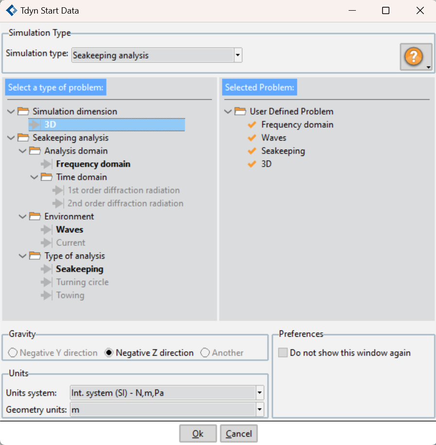
When starting up the Tdyn environment, the start data window will pop up. This window is meant to define the interface so that only those features that are necessary for the case study will be available. This way, the interface will show only those parameters and boundary conditions required, hiding those unnecessary, and therefore making it easier to use and navigate through.

The following figure shows the Tdyn environment and the start data window. In order to use SeaFEM, make sure that Seakeeping analysis option is selected from the Simulation type box.

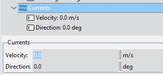
Within the Analysis domain section of the problem selection data tree you can select either frequency or time domain analysis. When selecting the frequency domain option, the remaining options are automatically set up. On the contrary, if the time domain option is selected, then first or second order diffraction radiation options can be choosen depending on the wave order you want to be used for the analysis. Furthermore, under the environment section of the data tree, you can select whether waves and/or currents are to be used. Finally, under the Type of analysis folder, the following three options are available:

• Seakeeping:this option will allow the user to activate body movements on those unrestrained degrees of freedoms.

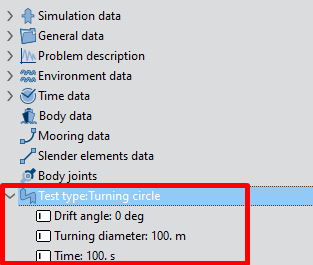
• Turning circle: this option is meant to simulate a body following a circular trajectory. Therefore, surge, sway and yaw will be restrained.

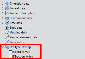
• Towing: this option is meant to simulate a ship following linear trajectory with a certain direction and speed. Therefore, surge, sway and yaw will be restrained.

It is obvious that Turning circle and Towing are not compatible options. On the other hand, any other combination of options are compatible simultaneously.

The Start data window can be accessed and modified at any time through the Data menu:

Data > Start data

or through the Data tree.

Fig. 1.38 Start Data window

1.4.2.2. General data

This section contains basic data necessary for simulating any kind of problem. The next figure shows the General data section in the Data tree as well as in the boxes underneath. Data can be modified in both locations, the data tree and in the boxes underneath when a specific section has been selected. It is divided into several sections described below:

Fig. 1.39 Tdyn data tree and General data panel

• Units: Set the type of units to be used.

• Gravity: Set the gravity value, the direction and the units.

• Water density: Set the water density and the metric unit.

• Problem setup: This section is equivalent to the start data window. Values can be modified though the start data or here.

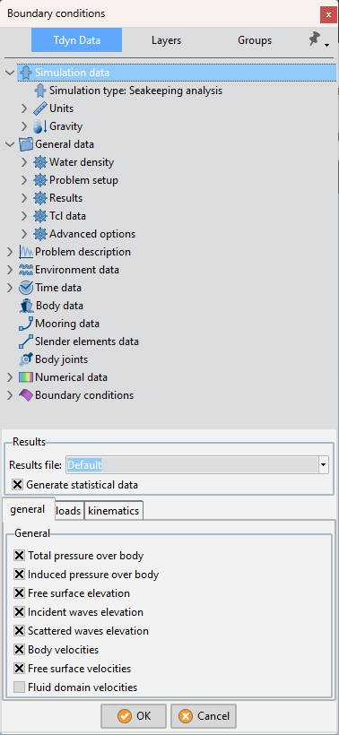
• Results: This section is meant to set what kind of results we want to obtain, and in which format they must be written. Note that if the frequency domain type of analysis is being used it is only necessary to specify the results file format. The rest of the options listed here are only available when a time domain analysis is undertaken.

  • Results file: select the format in which the results are to be written. Binary formats are less memory consuming. Binary 1 has to be selected if traditional GID post process is to be used. Binary 2 format (default) is to be used if the newer post process is to be used. Additionally, the native Nemoh file format is available for frequency domain analysis.

  • General: select those values to be written in the result files. The values shown under “general” are those field values over meshes. Then, they might cause the result fields to be quite large memory.

  • Loads: Forces and moments acting over the body under study can be recorded along the simulation. Pressure load refers to those loads obtained by integrating the pressure over the body surfaces. total loads refers to all kind of loads, including pressure loads, hydrostatic restoring loads, and any other external load brought into the simulation.

  • Kinematics: in this section, select the variables to be recorded during the simulation. Movements, velocities and accelerations are referred to the gravity center of the body. Raos stand for Response Amplitude operator.

  • User defined: Here, the user can create time dependent outputs. These outputs might be written analytically and might be dependent on any variable involve in the simulation, such as position, velocity or acceleration of the body, pressure over pressurized free surfaces, etc.

1.4.2.3. Problem description

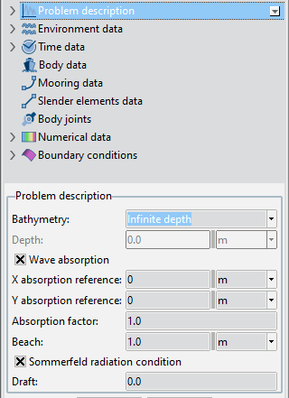
In this section, some key parameters necessary to carry out the simulation have to be provided. The following figure shows the data interface. Note that this section of the data tree becomes more simple when using the frequency domain type of analysis. In that case, only the type of bathymetry to be used (and optionally their corresponding depth) must be specified.

Fig. 1.40 Problem description data interface

Bathymetry:

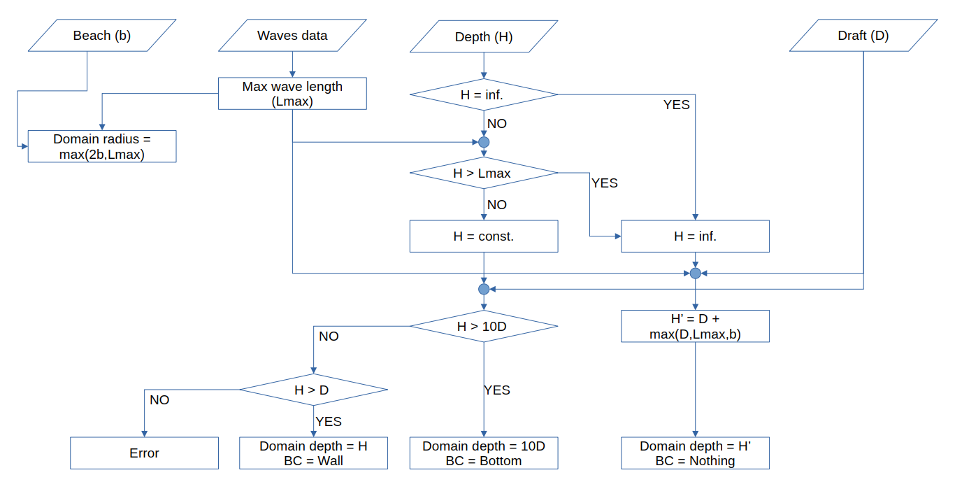
• Infinite depth: to be used when the depth is much larger than the wave lengths. In this case, the depth of the domain is recommended to be at least equal to half the wave length of the largest incident wave. However, smaller computational depths can be used in combination with the Bottom boundary condition to simulate lager depths. This can be done when de characteristic length of the body under analysis is small compared to the computational depth.

• Constant depth: to be used when the bottom is flat, and the depth is constant and smaller than half the wave lengths of the largest wave. Smaller computational depths can be used in combination with the Bottom boundary condition the same way it has been indicated previously.

• Depth: only available if Bathymetry=Constant depth was selected. The real depth of the problem must be introduced in the box

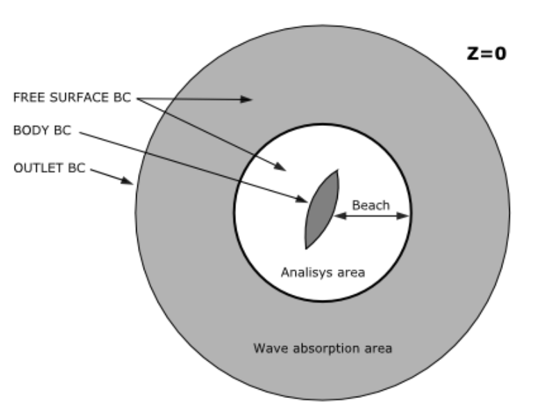
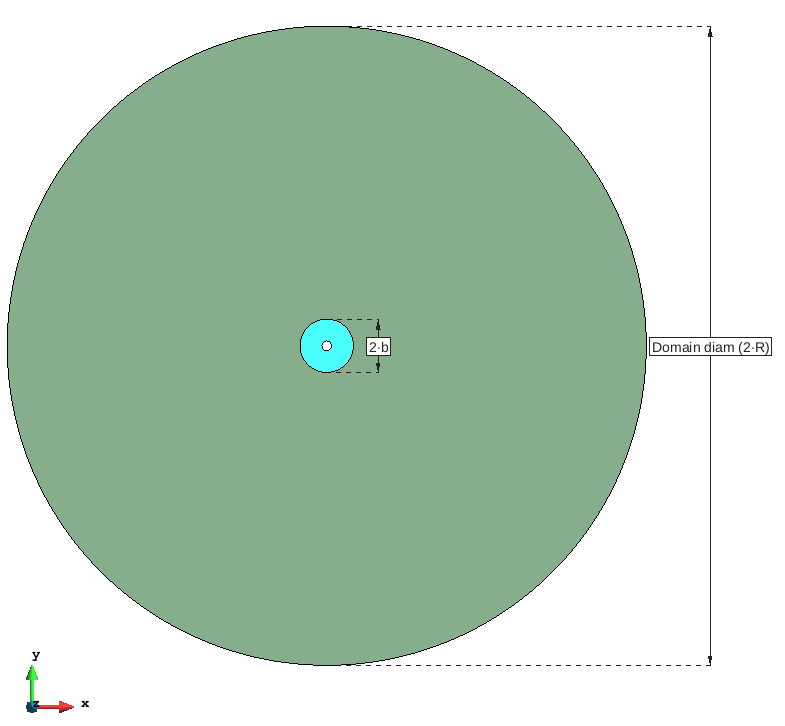
Wave absorption: select if scattered waves generated by the presence of the body are to be absorbed in order to avoid reflection at the edge of the computational domain. The absorption area will start at a specific distance (Beach)from a reference point located on the free surface. Therefore, there will be no absorption in the circle with center the reference point, and radius the value introduced in “Beach”. The area with no dissipation will be referred as the analysis area since no artificial dissipation is introduced on purpose to damp waves refracted and radiated by the body.

X absorption reference: X coordinate of the reference point to determine the analysis and absorption area.

Y absorption reference: Y coordinate of the reference point to determine the analysis and absorption area.

Absorption factor: determines how strong the dissipation is (recommended value “1”). Large absorption factors might cause instabilities and/or wave reflection. Smaller values, while being less likely to cause instabilities, but will require larger computational domains to damp refracted and radiated waves.

Beach: determine how far, from the reference point, the free surface absorption starts.

Sommerfeld radiation condition: This option is only available in those cases where the the body is subjected to waves, has no translational movement (turning circle/towing) and is in the absence of currents. In these cases, the largest waves can be hard to be dissipated in the absorption area unless a large computational domain is used. To avoid this situation, a Sommerfeld radiation condition can be used to allow the largest waves to leave the domain across the edge of the computational domain. Therefore, the combined action of the dissipation area and the Sommerfeld radiation condition is the best choice to avoid reflection of waves onto the edges.

Fig. 1.41 Analysis area and wave absorption area

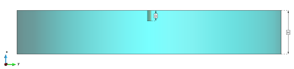
Draft: SeaFEM considers by default the free surface at the vertical position Z=0. Insert the draft in this field in order to run the analysis with the hull’s keel position at Z=0. As a consequence, the free surface level is updated to the draft.

1.4.2.4. Computational domain generation

1.4.2.4.1. Basic user input variables

The following basic user variables are necessary to define computational domain. They are explained in the previous section

• Beach:

• Waves data:

• Depth:

• Draft:

1.4.2.4.2. Domain dimensions

Fig. 1.42 Lateral view of domain dimensions. D: Draft, H: Depth

Fig. 1.43 Front view of domain dimensions. b: Beach

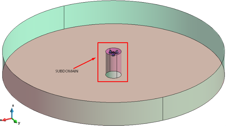
It is advised to build a subdomain (an internal concentric cylinder) for mesh refinement close to the floater and the free surface. The radius of this subdomain can be taken as the beach ().

Please take into account that both domain and subdomain volumes must share the inner contour surface, in order to share the mesh volume elements’ faces, and hence keep the mesh connection.

Fig. 1.44 Detail of the subdomain within the model domain

1.4.2.5. Environment data

This section aims to offer the data required for simulating the marine environment. Various options are available depending on whether frequency or time domain is being considered.

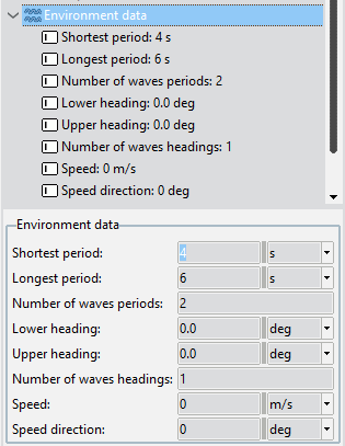
• Frequency domain:

  In this case, the wave spectra will be a set of monochromatic waves defined by the period and heading of each wave. The data to be inserted is quite simple and the user only needs to define the following inputs:

  • Shortest and Longest Period: Shortest and Longest wave periods that the wave spectra will have.

  • Number of waves periods: total number of wave periods to be used in the wave spectra.

  • Lower and Upper heading: Lower and Upper wave heading that the wave spectra will have.

  • Number of waves headings: Total number of wave headings to be used in the wave spectra.

  • Speed: Total forward speed that the bodies will have.

  • Speed direction: Direction of the speed for all bodies.

  

• Time domain:

  Different sort of wave spectra are available for time domain analyses, each one requiring of specific data. The wave spectra is introduced in SeaFEM as an incident velocity potential.

  

  

  Fig. 1.45 Environment data interface

  Wave environment data and currents environment data can be defined through the menu options:

  Environment data > Waves

  and

  Environment data > Currents

  respectively

1.4.2.5.1. Wave environment data

Next is a description of the different inputs to be provided by the user:

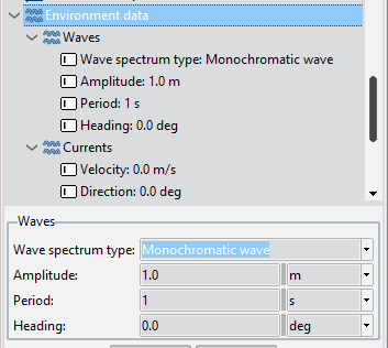
Wave spectrum type: select the type of incident wave environment. The following options are available.

• Monochromatic wave: this is the simplest spectrum available. This option generates an incident wave that corresponds to a monochromatic wave. In order to determine this monochromatic wave, the wave amplitude, period and direction of propagation must be provided.

  

  Fig. 1.46 Wave parameters

• Pearson Moskowitz spectrum:

  \[S( \omega ) = H^{2}_{s} \cdot T_{m}( \frac{0.11}{2 \pi } )( \frac{T_{m}}{T} )^{-5}exp[-0.44( \frac{T_{m}}{T} )^{-4}]\]

  where T is the wave period; H_sis the significant wave height; T_m is the mean wave period, which is obtained \(T_{m}=2 \pi m_{0}/m_{1}\), with \(m_{0}\) and \(m_{1}\) the zero and first moments of the wave spectrum. This is probably the simplest idealized spectrum, obtained by assuming a fully developed sea state, generated by wind blowing steadily for a long time over a large area. For further information, please refer to the SeaFEM Theory Manual.

• Jonswap2 spectrum: The JONSWAP spectrum was established during a joint research project, the “Joint North Sea WAve Project”. This is a peak-enhanced Pierson-Moskowitz spectrum given on the form

  \[S( \omega ) = \left( \frac{5}{16} \cdot H^{2}_{s} \cdot \frac{ \frac{T^{5}}{T^{4}_{p}} }{2 \pi} \right) \cdot e^{-1.25 (\frac{T_{p}}{T})^{-4}} \cdot (1-0.287 \cdot log(\gamma)) \cdot \gamma^{Y}\]
  \[Y=e^{-(\frac{0.159 \omega T_{p}-1}{ \sigma \sqrt{2}})}\]

  where \(\omega=2\pi/T,\sigma=0.07\) for \(\omega<=6.28/T_{p}\), \(\sigma=0.09\) for \(\omega>6.28/T_{m}\), T is the wave; H_sis the significant wave height, T_pis the peak wave period and \(\gamma\) is the peakedness parameter. For further information, please refer to the SeaFEM Theory Manual.

• Jonswap spectrum: An alternative definition of the JONSWAP spectrum given by

  \[S( \omega ) = \left( \frac{155H^{2}_{s}}{T^{4}_{m} \omega ^{5}} \right) \cdot e^{-944T^{-4}_{m} \omega ^{-4}} (3.3)^{Y}\]
  \[Y = e^{-( \frac{0.191 \omega T_{m} - 1}{ \sigma \sqrt{2}})^{2}}\]

  where \(\omega=2\pi/T,\sigma=0.07\) for \(\omega<=5.24/T_{m}\), \(\sigma=0.09\) for \(\omega>5.24/T_{m}\), T is the wave period; \(H_{s}\) is the significant wave height; \(T_{m}\) is the mean wave period, which is obtained via \(T_{m}=2\pi m_{0}/m_{1}\), with \(m_{0}\) and \(m_{1}\) the zero and first moments of the wave spectrum. For further information, please refer to the SeaFEM Theory Manual.

  • White noise: introduce a number of waves with frequencies uniformly distributed across an interval, and with same amplitude and direction. This spectrum is used to carry out response amplitude operator (RAO) analysis with the time-domain solver.

  • Customize: a spectrum can be defined based on the significant wave height and mean wave period.

  • Read from file: by using this option, any generic wave spectrum can be defined by the user. To this aim, a text file must be provided in the data tree entry that becomes available when rhe ‘Read from file’ option is selected. In the text file the user must indicate the relevant wave parameters (period T, amplitude A, wave direction G and wave phase P) for each wave component conforming the spectrum. The specific format of the wave spectrum file can be viewed in the following example.

    SeaFEM Spectrum_file version 1.0

    NWaveComponents 20

    TWaves AWaves GWaves PWaves

    14.6613 2.56028e-005 -0.349066 2.94053

    12.6662 0.000229263 -0.116355 3.14788

    13.7174 0.000229263 0.116355 4.55531

    11.8723 2.56028e-005 0.349066 2.25566

    7.21275 0.0123038 -0.349066 2.92168

    7.73874 0.110176 -0.116355 0.917345

    8.79714 0.110176 0.116355 5.20248

    7.21466 0.0123038 0.349066 3.09133

    5.66508 0.0427017 -0.349066 5.92504

    5.86992 0.382376 -0.116355 2.74575

    6.4778 0.382376 0.116355 3.80133

    5.77667 0.0427017 0.349066 0.967611

    5.33589 0.0272918 -0.349066 2.40646

    5.20454 0.244386 -0.116355 4.50504

    4.92538 0.244386 0.116355 5.62973

    5.17884 0.0272918 0.349066 4.56788

    4.13839 0.0189668 -0.349066 3.38664

    4.07775 0.16984 -0.116355 5.73655

    4.20474 0.16984 0.116355 1.88496

    4.65867 0.0189668 0.349066 5.62345

    This user defined spectrum file is equivalent to a Jonswap spectrum realization with the following characteristics:

    • Mean wave period = 5 sec.

    • Significant wave height = 2 m.

    • Shortest period = 4 sec.

    • Longest period = 15 sec.

    • Number of wave periods = 5

    • Mean wave direction = 0 deg.

    • Spreading angle = 40 deg.

    • Number of wave directions = 4

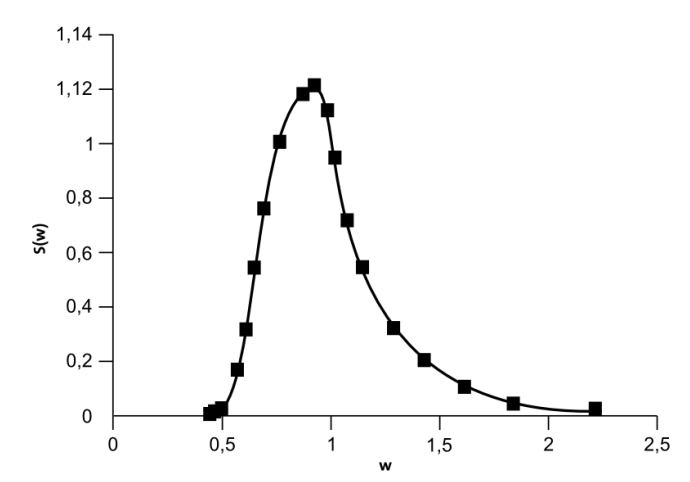
• Customize spectrum: if the option “customize” has been selected in “Wave spectrum type”, the user can introduced a spectrum based on the significant wave height and mean wave period. For instance, a Pearson Moskowitz spectrum could be written as follows:

  \[(H^{2}_{s} \cdot T_{m}) \cdot \frac{0.11}{2 \cdot \pi} \cdot \left( \omega_{s} \cdot \frac{T_{m}}{2 \cdot \pi} \right)^{-5} \cdot e^{-0.44 \cdot ( \omega_{s} \cdot \frac{T_{m}}{2 \cdot \pi} )^{-4} }\]

  where \(H_{s}\) represents the significant wave height; \(T_{m}\) represents the mean wave period, \(\omega_{s}\) represent the wave frequency \(\omega=2\pi/T\) (See appendix A).

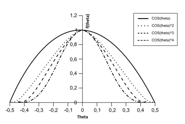
• Directional wave energy: this variable allows the introduction of a directional wave energy distribution \(f(\theta)\), aiming to reproduce spectra with higher energy around the mean direction of propagation, and decaying as the direction diverge from the mean A typical directional wave energy distribution can be expressed as:

  \[f(\theta) = cos^{2}(\frac{2 \theta}{3}), where \theta = \pi \cdot \frac{\gamma-\gamma_{m}}{\gamma_{max}-\gamma_{min}} cos^{2}(\frac{2}{3} \cdot \gamma_{s} \cdot \pi)\]

  and θ goes from -π/2 to π/2. This directional energy distribution should be introduced with the following syntax:

  

  Fig. 1.47 Directional wave energy Examples

• Amplitude: amplitude of monochromatic wave or amplitude for white noise spectrum waves.

• Period: period of the monochromatic wave.

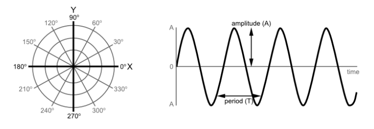
• Heading: direction of the monochromatic wave or direction for white noise spectrum waves. The wave heading (direction) is defined as the angle from the positive global X axis to the direction in which the wave is travelling, measured anticlockwise when seen from above. Therefore waves travelling along the X axis (from -X to +X) have a 0 degree wave direction, and waves travelling along the Y axis (from -Y to +Y) have a 90 degree wave direction.

• Mean wave period: mean wave period for wave spectrum such as Pearson Moskowitz, Jonswap, etc.

• Significant height: significant wave period for wave spectrum such as Pearson Moskowitz, Jonswap, etc.

• Shortest period: correspond to the wave with maximum frequency to be considered when discretizing a spectrum. Tmin=Tm/2.2 recommended.

• Longest period: correspond to the wave with minimum frequency to be considered when discretizing a spectrum. Tmax=2.2Tm recommended.

• Number of wave periods: or number of wave frequencies to be used.

• Mean wave heading: mean direction of wave propagation. It is provided in the form of an angle θ measured with respect to the X global axis. The wave heading (direction) is defined as the angle from the positive global X axis to the direction in which the wave is travelling, measured anti-clockwise when seen from above. Therefore waves travelling along the X axis (from -X to +X) have a 0 degree wave direction, and waves travelling along the Y axis (from -Y to +Y) have a 90 degree wave direction.

• Spreading angle: angular sector Δθ within which the waves propagate. Such an angular sector is always centered at the mean wave heading so that the waves propagate within the range [θ - Δθ/2, θ + Δθ/2]

• Number of wave headings: in case the waves propagate within an angular sector specified by the mean wave heading and the spreading angle, this parameter determines how many directions such an angular sector will be discretized into.

• Realization repeatibility: this option must be activated if the user wishes to run exactly the same spectrum realization in further simulations. By contrast, if such an option remains deactivated, random realizations of the same given spectrum will be used when running the simulation several times.

  Note: the total number of waves used in the realization will be the “number of wave periods” times ”Number of wave directions”.

  

  Fig. 1.48 Pearson Moskowitz discretization. Hs=1; Tm=1; Tmax=2.2Tm; Tmin=Tm/2.2; N=20

1.4.2.5.2. Currents environment data

Next is a description of the various inputs to be provided by the user when using currents:

• Velocity: velocity of the water current.

• Direction: direction of the water current.

1.4.2.6. Time data

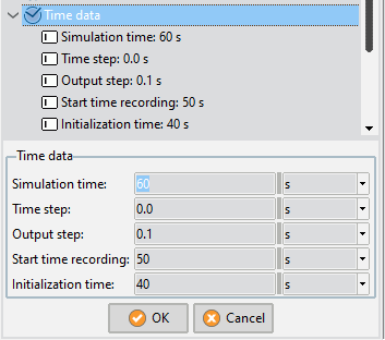
In this section, several parameters regarding the timing of the simulation are to be defined. Note that time data presented in this section only concern to time domain analysis but not frequency domain.

Fig. 1.49 Time data interface

• Simulation time: length in time of the simulation.

• Time step: time step to be use for the time marching schemes. The time step introduced in this box will be the one used unless a zero value is introduced. If a zero value is introduced, the time step will be internally calculated by SeaFEM based on the minimum mesh size and the stability parameter β=g∆t2/∆zmin.

• Output step: time lag between recordings. Values corresponding between two time steps are linearly interpolated between the previous and the next time step.

• Start time recording: set the point in time when the writing of the results will start.

• Initialization time: set an initialization time period. During this period, the wave amplitudes and currents will be increased smoothly from zero to their final values following this expression: \(Initialization factor = 0.5·(1-cos( \pi ·time/time_{init}))\). This initialization process is meant to avoid long transient behaviours due to sudden initializations. Sudden initializations may lead to an unrealistic and highly energetic transient behaviours. In this cases, longer simulations are required so the unrealistic high energy behaviour will dissipate over time.

1.4.2.7. Numerical data

As well as the time data presented in the previous section of the manual, numerical data shown herein concerns only time domain analysis.

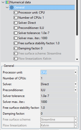
The Numerical data section of the SeaFEM data tree collects information concerning the numerical algorithms underlying the SeaFEM solver. Most of the computational time required by SeaFEM is spent in solving the linear system of equations resulting from the discretization of the governing equations. Therefore, selecting the correct parameters will enhance having faster and even more accurate simulations. Numerical parameters that affect the behavior and performance of the main SeaFEM solver (that devoted to solve the finite element based potential flow problem) appear within the General subsection of the SeaFEM data tree. On the other hand, numerical parameters related to the multi-body dynamics solver are collected within the Body dynamics subsection of the SeaFEM data tree.

Fig. 1.50 Numerical data > General

Fig. 1.51 Numerical data > Body dynamics

A brief description of the meaning of each numerical parameter and the possible values they can take is provided in the following list:

1.4.2.7.1. General numerical data

• Processor Unit: while most part of the computations are carried out by the CPU, SeaFEM provides the option of solving the linear system of equations faster by means of the graphic processor unit (GPU). Since most of the computational time is spent in solving these linear systems, GPU provides a way to speed up our SeaFEM computational time. Any GPU device supporting CUDA and double precision is suitable of being used (see developer.nvidia.com for further information).

  • CPU: all computations are carried out in the CPU.

  • CPU+GPU: linear systems of equations concerning the main SeaFEM problem are solved in the GPU. Any other computation, as for instance the solution of the body dynamic’s problem is carried out in the CPU.

• Number of CPUs: those calculations carried out in the CPU may take advantage of the multithread parallel computing capabilities of modern processors. The number of CPUs indicates how many of the available computer’s processors are going to be used during the calculation.

• Solver: these is the list of available solvers. It actually depends on the type of analysis under consideration. In those cases where either current or body translational movements (turning circle/towing simulations) are present, only Stab-BiCG and Direct solvers are available. When neither currents nor translational movements exist, the complete list of solvers becomes available. When the CPU+GPU option is being used, the Direct solver is not available in any case.

  • Conjugate gradient: iterative solver suitable to solve problems leading to a linear set of algebraic equations with a symmetric matrix structure

  • Bi-conjugate gradient: iterative solver suitable to solve problems leading to a linear set of algebraic equations with a non-symmetric matrix structure.

  • Stab bi-conjugate gradient: modified version of the biconjugate gradient solver that can provide more stability in some ill-posed numerical problems.

  • Deflated conjugate gradient: deflated version of the conjugate gradient iterative solver. Be aware that the deflation process is not always guaranteed to speed up the solving process. Based on our experience, most of the time it does, but care must be taken when selecting this option. If you feel that SeaFEM is running slow under this option, stop the calculation and select the CG solver instead, compare the speed of the simulation, and act consequently.

  • Direct: direct solver based on the third-party IntelMKL numerical solvers library.

• Preconditioner: these is the list of available preconditioners to be used in conjunction with the iterative solvers listed above in order to speed-up the calculations.

  • if the Processor Unit is set to CPU, the ILU preconditioner is recommended.

  • if the Processor Unit is set to CPU + GPU and neither currents nor translational movements are simulated: the SPAI preconditioner is recommended.

  • if the Processor Unit is set to CPU + GPU and either currents or translational movements are simulated: the Diagonal preconditioner is recommended.

• Solver tolerance: maximum tolerance allowed to reach convergence when using iterative solvers. The default value \(10^{-7}\) is recommended.

• Solver max iterations: maximum number of iterations to be carried out by the solver until convergence is achieved. The default value 1000 is recommended.

• Free surface stability factor: this factor controls the time step as explained in the time data section, unless a positive time step has been prescribed. If neither currents nor translational movements are simulated, typical values for stability are in the order of 1. If either currents or translational movements are simulated, typical values for stability are in the order of 0.1-0.001, depending on the Froude number. The larger the froude number, the smaller the stability parameter and the time step.

• Damping factor: this parameter is available in those cases where the body under study has unrestrained degrees of freedom. Sometimes, the only mechanism to dissipate energy by the body is through wave radiation. However, this mechanism might not be dissipative enough and might cause very long transient periods due to its low dissipation capabilities. This might be a problem specially when the body is excited with waves whose frequencies are near the resonance frequency of the body. This problem can be mitigated by introducing a small dissipation which is only noticeable near resonance. This is carried out by bringing a percentage of the critical damping into the dynamic equations of the body. It is recommended to use this option only in those cases where it is necessary due to the low wave radiation capacity of the body, and where the body is excited near its resonance frequency. Values between 0 and 0.05 are recommended, depending on the case.

• Free surface scheme: this option is only available when either currents or translational movements exist. This parameter actually determines the numerical scheme to be used when solving the free surface boundary condition with convective terms.

  • Streamlines: in this case, the convective term of the free surface boundary condition is obtained by using a streamline differential operator that actually uses two points upstream and one point downstream to evaluate the derivatives along the streamline.

  • FEM SUPG: this is an alternative method for the integration of the free surface boundary condition. In this case a finite element based SUPG stabilization scheme is used.

• Flow linearization: this option is only available when either currents or translational movements exist. It specifies the type of linearization to be used when integrating the convective terms within the free surface boundary condition.

  • Kelvin: flow around the body is assumed as if is not perturbed by the presence of the body.

  • Slow Kelvin: Kelvin linearization above is used but convective terms in the free surface are not taken into account.

  • Double body: flow around the body is assumed as if the free surface behaves as a wall.

  • Slow double body: double body linearization above is used but convective terms in the free surface are not taken into account.

  • Non-linear: flow around the body is continously updated to take into account the presence of the body and the effects of waves generated at the free surface.

1.4.2.7.2. Body dynamics numerical data

• Dynamic solver max. iterations: maximum number of iterations allowed for the dynamic solver.

• Dynamic solver relaxation: this parameter concerns the numerical relaxation of the dynamic solver. It must be greater than cero.

• Max iterations time step: This parameter is available in those cases where the body under study has unrestrained degrees of freedom. In these cases, an iterative procedure must be carried out within each time step to reach convergence of the body dynamics driven by the hydrodynamic and external loads acting on the body. This parameter sets the maximum number of iterations allowed per time step until convergence is achieved.

• Tolerance: maximum tolerance allowed to reach convergence in the iterative procedure carried out within each time step.

• Alpha B-N: this parameter concerns the stability of the Bossak-Newmark scheme used to solve the multibody dynamics system. It usually takes a negative value. A positive value may be advisable when the time step is very small since in this case a first order scheme can increase stability while precision is preserved inherently because of the small value of the time step.

• Large displacements: this option must be activated to take into account large displacements when solving the multi-body dynamics system. If this option is active, the inertia matrix of the bodies is updated every time step to take into account the finite rotation of the body. Forces and moments are updated as well to take into account this effect. Note that large displacements have limited application within SeaFEM since the actual position of the body regarding the incident wave is not updated. Hence, caution is adviced when interpreting the results obtained using the large displacements option.

1.4.2.8. Body data

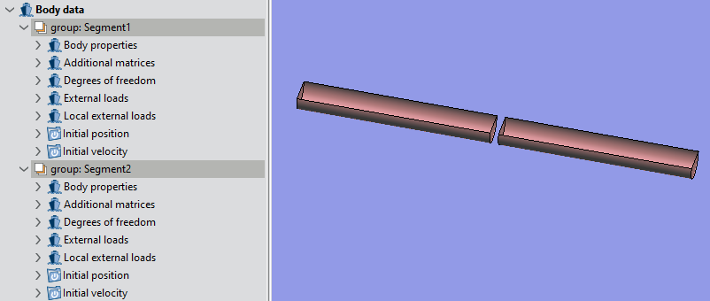
Body Data section is intended to allow the user to define several bodies and their corresponding properties. The user can create as many bodies as necessary, each one being assigned to a different group of geometrical entities. In the figure below for example, two different bodies have been defined, each one being assigned to a different cylindrical floating body.

Fig. 1.52 Multiple bodies defined through the GUI

For each body, information regarding the mass and the radii’s of inertia and unrestrained degrees of freedom must be provided. This is so irrespectively of wether frequency or time domain options are under consideration. If a time domain calculation is undertaken, additional external forces and moments can be defined for each body.

Fig. 1.53 Body data definition window

Each body data section is described in detail in what follows.

1.4.2.8.1. Body properties

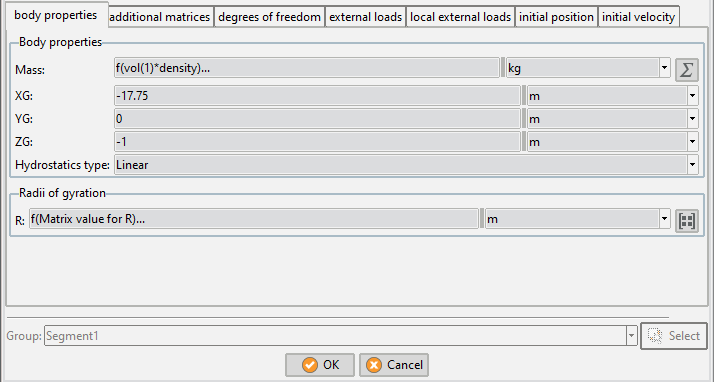
Basic data regarding the body must be provided in order to solve the body’s dynamics if the body has unrestrained degrees of freedom.

To define body properties use the menu option:

Body data > Body properties

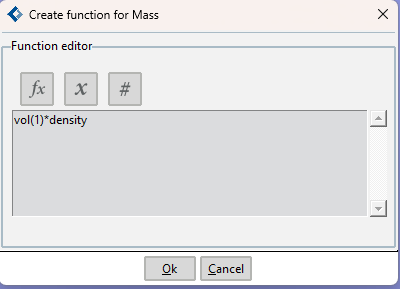
• Mass: the body mass can be introduced in two different ways: either introducing the exact value or using the function editor. When using the function editor, the mass can be calculated as an analytical value depending of some variables used by SeaFEM. For example, for freely floating objects where the mas must equal the mass of the displaced water, we could write \(Mass=volume·density\), where volume refers to the displaced water volume, and density refers to the water density. This specific case is shown in the following figure.

  

  Fig. 1.54 Mass function editor

• XG: introduce the x coordinate of the gravity center of the body.

• YG: introduce the y coordinate of the gravity center of the body.

• ZG: introduce the z coordinate of the gravity center of the body.

• Hydrostatic type: this parameter has two possible values, Linear and Non-Linear.

  By default, the linear option is used so that the calculation of the hydrostatic recovery forces is linearized. By doing this, the displacements of the floating structure are assumed to be small and the hydrostatic restoration coefficients assumed to be constant. This allows for the coefficients to be calculated just once at the beginning of the simulation taking into account the initial configuration.

  By using the non-linear option, the hydrostatic restoration coefficients are assumed to depend on the actual movement of the floating structure and they must be evaluated at each time step. To this aim, an auxiliary body mesh (containing the entire body) is necessary for tracking the actual position of the body surface during the simulation, thus allowing for the proper integration of the hydrostatic pressure. Such an auxiliary mesh must be generated for each body under analysis and exported in a text file using GiD mesh format. The generated mesh file must be provided as “Body mesh” option under Body properties.

  The Non-Linear hydrostatic type option allows for the simulation of those phenomena that are inherently non-linear as for instance the parametric resonance.

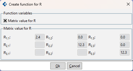
• Radii of gyration: the elements of the inertial matrix are related to the radii of gyration as: \(Iii=Mass·rii·rii; Pij=Mass·rij·|rij|\). Then:

  • rxx: \(r_{xx} = \sqrt{ \frac{I_{xx}}{Mass} }\)

  • rxy: \(r_{xy} = \left( \frac{P_{xy}}{|P_{xy}|} \right) \cdot \sqrt{ \frac{|P_{xy}|}{Mass} }\)

  • rxz: \(r_{xz} = \left( \frac{P_{xz}}{|P_{xz}|} \right) \cdot \sqrt{ \frac{|P_{xz}|}{Mass} }\)

  • ryy: \(r_{yy} = \sqrt{ \frac{I_{yy}}{Mass} }\)

  • ryz: \(r_{yz} = \left( \frac{P_{yz}}{|P_{yz}|} \right) \cdot \sqrt{ \frac{|P_{yz}|}{Mass} }\)

  • rzz: \(r_{zz} = \sqrt{ \frac{I_{zz}}{Mass} }\)

Fig. 1.55 Radii of gyration matrix interface

1.4.2.8.2. Additional matrices

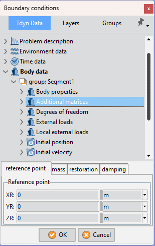
The Additional matrices option can be used to provide additional mass, restoration and damping matrices for the body under consideration. This can be useful when we want to take into consideration mass, stiffness and damping effects different from the hydrodynamic effects directly accounted for by SeaFEM’s solver. This is the case, for instance, when parts of the body located above the free surface may be anticipated to suffer significant aerodynamic forces affecting the dynamics of the whole system. A typical example is the dynamic effect of the wind turbine attached to a floating TLP structure (see SeaFEM’s tutorials manual for further details on this example).

In these cases, a single mass, restoration and damping matrix can be specified for each body through the data tree’s GUI, as shown in the following figure.

Fig. 1.56 Additional matrices option as it appears in the SeaFEM’s data tree. As can be seen, a reference point must be provided.

If more than one individual matrix needs to be provided, it can still be done by using the SeaFEM’s TCL extension. In this case, an index identifying the body to which the matrix is associated and the corresponding reference point must be provided for each individual matrix (see also SeaFEM’s tutorials manual for further details on this usage). The actual syntax looks like this:

TdynTcl_Add_Mass_Matrix <bIdx> [list <xcoord> <ycoord> <zcoord>]
[list <M11> <M12> ... <M66>]

where <bIdx> is the index thats identifies the body, <xcoord>, <ycoord>, <zcoord> are the coordinates of the reference point and <M11> … <M66> are the 36 coefficients of the matrix.

Similarly, the TCL’s extension syntax for additional stiffness and damping matrixes reads as follows.

TdynTcl_Add_Stiffness_Matrix  <bIdx>  [list  <xcoord>  <ycoord>
<zcoord>] [list <S11> <S12> ... <S66>]
TdynTcl_Add_Damping_Matrix  <bIdx>  [list  <xcoord>  <ycoord>
<zcoord>] [list <D11> <D12> ... <D66>]

Managing an arbitrary reference point

It has already been noted that a reference point, to which the matrix coefficients are referred, must be provided for all additional matrices. With this information, SeaFEM internally evaluates the actual position of the gravity center of the body system and transforms the matrices so that they are all referred to the new gravity center. Note that such an internally updated gravity center may not coincide in general with that specified by the user in the “Body properties” tab that actually corresponds to the reference point of the body’s main component. In any case, the actual position of the gravity center of the system is output for each body at the beginning of the information file when running the simulation. Finally, the dynamics of the system are finally solved in the body’s frame of reference so that all the results are referenced to the corresponding updated gravity center.

Sometimes it can be useful to set the mass of the body to zero and actually enforce the mass and inertia properties of the body by using the additional mass matrix option. If this is the case, the radii of gyration data in the Body properties section of the data tree has no effect since the corresponding inertia coefficients evaluate to zero (i.e. \(I_{ij} = R_{ij}^{2}·M\) being M equal zero) and the actual inertia matrix corresponds to that provided by the additional mass matrix option. Note that in the case of using the frequency domain module of SeaFEM, setting the mass of the body to zero has the effect of the solver to internally compute the actual mass of the body from the displacement and the water density. This is equivalent to what is done when using the time domain module if the “vol*density” formula is used in the “Mass” field of the body properties data.

1.4.2.8.3. Degrees of freedom

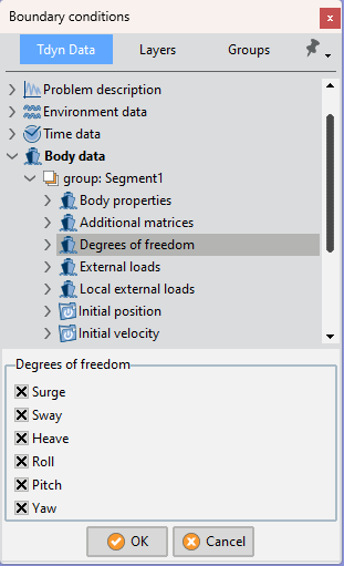
Next figure shows the interface where the user can activate/deactivate the unrestrained degrees of freedom. When performing analysis such as Turning circle or Towing, the Surge,Sway and Yaw are restrained degrees of freedom since the body is forced to follow a specific trajectory, while the Heave, Roll and Pitch are unrestrained.

Fig. 1.57 Degrees of freedom interface.

Degrees of freedom can be activated/deactivated through the menu option:

Body data > Degrees of freedom

• Surge: select if the floating object is supposed to translate along the x axis.

• Sway: select if the floating object is supposed to translate along the y axis.

• Heave: select if the floating object is supposed to translate along the z axis.

• Roll: select if the floating object is supposed to rotate around the x axis.

• Pitch: select if the floating object is supposed to rotate around the y axis.

• Yaw: select if the floating object is supposed to rotate around the z axis.

1.4.2.8.4. External loads

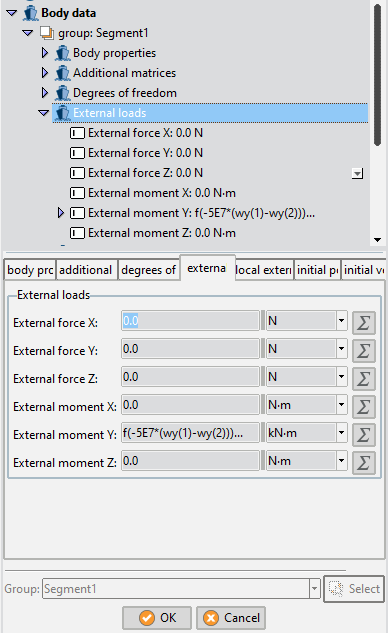
External loads (forces and moments) can be defined either as a constant value or via a set of analytical functions. This functions can be tuned to model, for instance, tension legs acting as springs. These external loads may be dependent on any of the variables listed in Appendix A.

Fig. 1.58 External loads interface

External loads can be defined using the menu option:

Body data > External loads

1.4.2.8.5. Local external loads

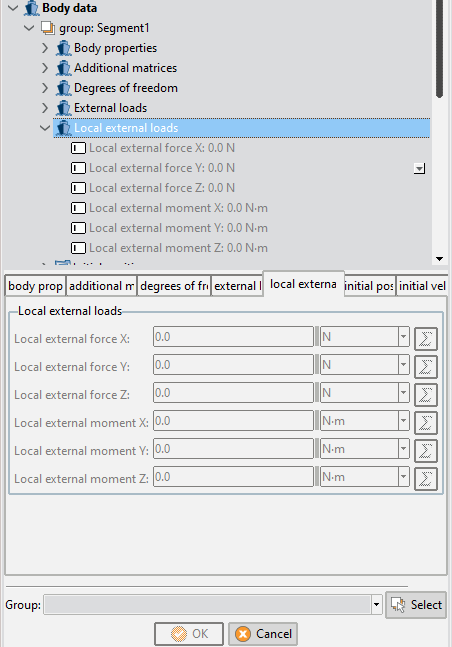
External loads (forces and moments) can also be defined relative to a local reference frame fixed to the body. This can be useful, for instance, to model the action of a PTO system when the displacements of the bodies cannot be considered to be small.

Local external loads can be defined either as a constant value or via a set of analytical functions. These external loads may be dependent on any of the variables listed in Appendix A.

Fig. 1.59 Local external loads interface

Body data > Local external loads

1.4.2.8.6. Initial conditions

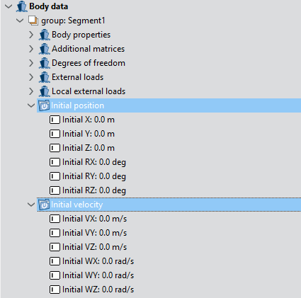
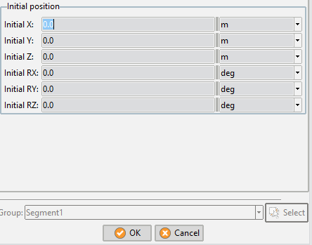
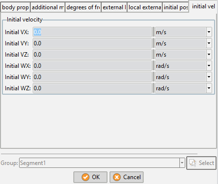
This section is used to introduced initial conditions for each body under analysis. For instance, if a extinction test in roll is to be carried out, the initial roll angle has to be known and introduced in the corresponding box. Initial velocities are applied in a similar way.

Fig. 1.60 Initial conditions

Initial Position Initial position options are available through the menu:

Body data > Initial position

• Initial X: set a initial X position for the object.

• Initial Y: set a initial Y position for the object.

• Initial Z: set a initial Z position for the object.

• Initial RX: set a initial RX rotation angle for the object.

• Initial RY: set a initial RY rotation angle for the object.

• Initial RZ: set a initial RZ rotation angle for the object.

Fig. 1.61 Initial position interface

Initial Velocity Initial velocity options are available through the menu:

Body data > Initial velocity

• Initial VX: set a initial X position for the object.

• Initial VY: set a initial Y position for the object.

• Initial VZ: set a initial Z position for the object.

• Initial WX: set a initial RX rotation angle for the object.

• Initial WY: set a initial RY rotation angle for the object.

• Initial WZ: set a initial RZ rotation angle for the object.

Fig. 1.62 Initial velocity interface

1.4.2.9. Mooring data

This section is devoted to present the GUI options available in SeaFEM to define a wide variety of mooring systems. All the information presented in this section is complementary to that in sections Appendix B: Tcl extension and Appendix E: Mooring definition by Tcl where the definition of mooring systems by using the Tcl extension of SeaFEM is described.

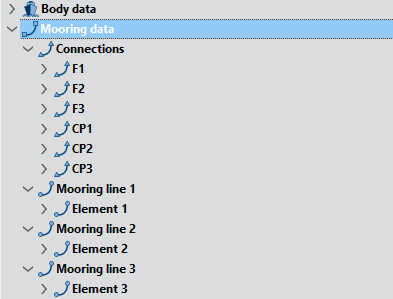
Mooring lines definition

A mooring system may consist on several independent mooring lines connected to a given body. At the same time, each mooring line may consist on several interconnected mooring segments (also called elements within the GUI). Elements (i.e. mooring segments) are linked at connection points (also called connections within the GUI). The image below shows an example of mooring system definition. In this case, the system consists on a single mooring line composed by three mooring segments (E11, E12, E14). The segments are connected between themselves, but also with the seabed and with the floating body through the connections points (P11, P12, …, P15).

Fig. 1.63 Mooring line.

New mooring lines can be created by right-clicking over the “Mooring data” option of the data tree and selecting the option “Create a new mooring line”. By default, when creating a new mooring line it contains a single element.

Mooring data > Create new mooring line

Elements definition

When creating a new mooring line, a single mooring segment is created by default and assigned to the current segment. New mooring segments can be created by copying the previous one and editing the corresponding parameters as they are described in what follows:

Fig. 1.64 Mooring element interface.

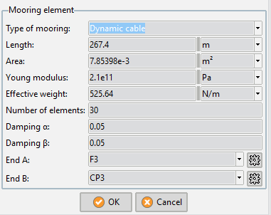
• Type of mooring: this parameter determines the type of mooring segment to be used. The possible values of this parameter are:

  • Spring: quasi-static elastic bar (spring able to work in both, tension and compression regimes).

  • Spring only tension : quasi-static cable (spring able to work only in tension)

  • Catenary : quasi-static elastic catenary

  • Dynamic cable : dynamic cable.

• Length [m] : length of the current mooring element

• Area [m:sup:`2`] : cross section area of the element

• Young modulus [Pa] : Young modulus of the current mooring element

• Effective weight [N/m] : effective weight (actual weight minus bouyancy) per unit length

• End A: This field is used to specify the first end point of the current mooring segment. It can be specified by either giving the coordinates of a new point, or by selecting an already existing point of the actual geometry. (See the “Connection definition” section below).

• End B: This field is used to specify the second end point of the current mooring segment. It can be specified by either giving the coordinates of a new point, or by selecting an already existing point of the actual geometry. (See the “Connection definition” section below).

• Number of elements : this parameter is only enabled when the dynamic FEM cable type of mooring is selected. It determines the number of line elements used in the cable discretization.

• Damping a, b : user defined damping ratios for dynamic cables

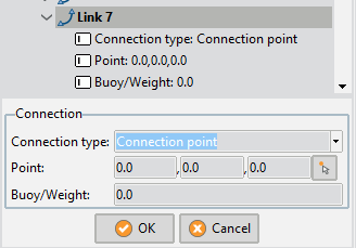
Connections definition

As it was shown in the previous section, any mooring segment must be defined by specifying the two end points (End A and End B) of the segment’s initial configuration. New connection points can be created in-situ when editing a given mooring element. If the connection point already exists, it will be available from the drop-down list next to the End A and End B entries in the “Mooring element” definition window. The next figures show the connection’s definition window that is used to define a new connection point. Specific parameters depend on the actual type of connection point being defined.

Fig. 1.65 Connection definition: connection point

Fig. 1.66 Connection definition: fairlead point

Fig. 1.67 Connection definition: anchor point

The required parameters and their possible values are described next.

• Name : name used to identify the connection point.

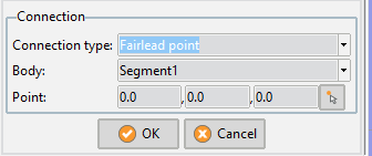
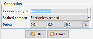
• Typetype of connection point.

  • Connection point: connection point used to link two mooring segments

  • Fairlead point: connection point used to link a mooring segment with a body

  • Anchor point: connection point used to link a mooring segment with the seabed

• Point : coordinates of the connection point

• Buoy/Weight : buoyancy or weight force to be applied vertically at the connection point. This parameter is available only for connection points between mooring segments

• Body: it determines to which body the mooring segment is linked to when using the current connection point. This parameter is only available for fairlead connection points.

• Seabed contact: type of interaction between the seabed and the mooring segment that ends at the current connection point. This parameter is only available for anchor connection points, and has effect only when using catenary mooring segments and cables. Possible values for this parameter are as follows:

  • Frictionless seabed

  • Chain with sandy seabed

  • Chain with mud/sand seabed

  • Chain with mud/clay seabed

  • Wire rope with sandy seabed

  • Wire rope with mud/sand seabed

  • Wire rope with mud/clay seabed

1.4.2.10. Slender elements data

This section is devoted to present the GUI options available in SeaFEM to define slender elements (i.e. Morison’s elements). All the information presented in this section is complementary to that in sections Appendix B: Tcl extension and Appendix F: Morison’s forces effect where the definition of slender elements by using the Tcl extension of SeaFEM is described.

Defining slender element sets

When viscous effects are anticipated to play a role on the dynamic behavior of an offshore structure, Morison’s equation can be used in SeaFEM to introduce force corrections due to such viscous effects. To this aim slender elements must be created and associated to a given body. For the sake of visual organization, such elements can also be grouped in the GUI of SeaFEM forming element sets . Based on the information provided by the user, SeaFEM evaluates Morison’s forces per unit length acting on each element, and after integration along the elements, the resultant forces are incorporated to the dynamics of the rigid body system.

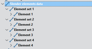
The image below shows an example of elements sets definition. In this case, the system consists on four element sets composed by one slender element each other.

Fig. 1.68 Slender element sets

Note that grouping slender elements in element sets has no special meaning and may be used only for organization purposes. But each individual element must be explicitly associated to a given body. New slender element sets can be created by right-clicking over the “Slender elements data” option of the data tree and selecting the option “Create new slender element set”. By default, when creating a new set it contains a single element.

Slender elements data > Create new slender elements set

Slender elements definition

When creating a new slender elements set, a single slender element is created by default and assigned to the current set. New slender elements can be created by copying the previous one and editing the corresponding parameters as they are described in what follows:

Fig. 1.69 Slender creation

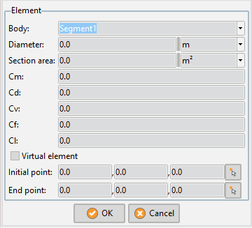
• Body: this parameter identifies the body to which the slender element is going to be connected.

• Diameter: diameter of the slender element cross section. Section area: total cross section area of the element.

• Cm: added mass correction coefficient.

• Cd: non-linear drag coefficient.

• Cv: linear drag coefficient.

• Cf: friction coefficient.

• Cl: lift coefficient.

• Virtual element: this parameter determines if the corresponding slender element is going to be considered a virtual element. If the virtual element option is checked floatability forces over the element are neglected.

• Initial point: coordinates of the point where the element begins.

• End point: coordinates of the end point of the element.

1.4.2.11. Test type

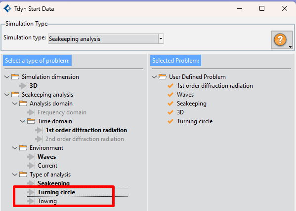
Test type data will be available in the SeaFEM data tree when either ‘Turning circle’ or ‘Towing’ type of analysis are selected. Note that these type of analysis are only compatible with the time domain type of problem.

Fig. 1.70 Test type is available when Turning circle or Towing is selected in Start data window.

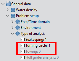
Type of analysis is also available through the menu

General data > Problem setup > Type of Analysis

Fig. 1.71 Turning circle or Towing are also available in Tdyn data tree.

Fig. 1.72 Turning circle test type options

Fig. 1.73 Towing test type options

Next is a description of the different inputs to be provided by the user depending on the test type being considered.

• Towing test type:

  • Speed: towing velocity applied during the test.

  • Direction: direction along which the towing velocity is applied. It is provided in the form of an angle measured with respect to the X global axis.

• Turning circle test type:

  • Drift angle: maneuver drift. It is provided in the form of an angle measured with respect to the X global axis.

  • Turning diameter: diameter of the turning circle of the test. It must be a positive number.

  • Time: time used to complete the maneuver.

1.4.2.12. Boundary conditions

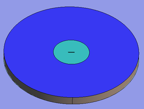
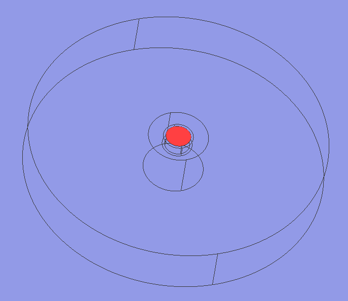
For time domain analysis, boundary conditions must be applied on the surfaces surrounding the volume, so the stated problem can be solved. Different type of boundary conditions can be applied, each of them aiming at different purposes. In order to explain each boundary conditions, the case study of a floating cylinder will be used as an example (see Application example section for further information). The following figure shows the geometry for this specific case study:

Fig. 1.74 Computational domain

Fig. 1.75 Boundary conditions interface

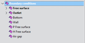
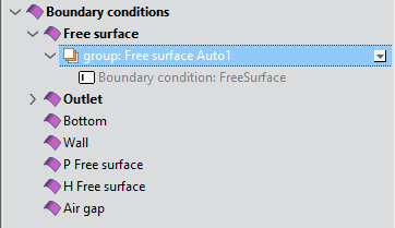
• Free Surface: Condition to be applied on the surfaces located at the plane z=0. On this surfaces, the kinematic and dynamic free surface boundary conditions will be applied.

  

  Fig. 1.76 Free surface interface

  

  Fig. 1.77 Free surface geometry

• Outlet: Condition to be applied to the vertical surfaces bounding the computational domain. It is used to apply two types of condition:

  • Case 1: this case has neither body translational velocities nor currents. Then the Sommerfeld radiation condition is applied for the longest waves.

  • Case 2: this case has body translational velocities and/or currents. Then no flow boundary condition for the scattered velocity potential is applied.

  

  Fig. 1.78 Outlet data interface

  

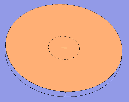
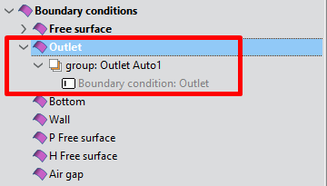
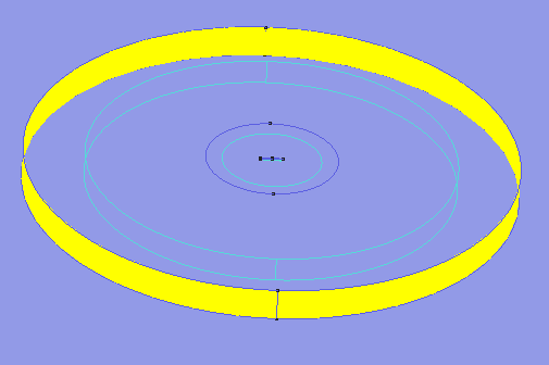
  Fig. 1.79 Outlet geometry where the boundary condition has been applied

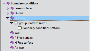
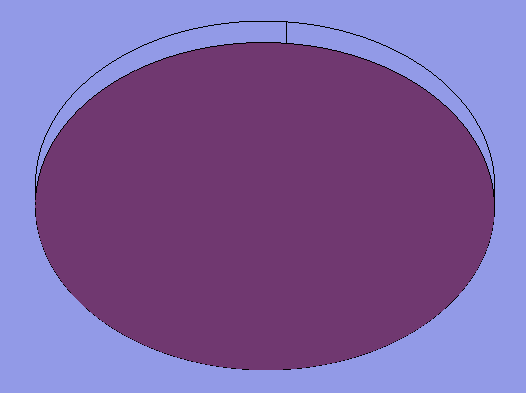
• Bottom: Condition to be applied to the lower horizontal surface bounding the computational domain. It is used to apply two types of conditions:

  • Case 1: this case has neither body translational velocities nor currents. Then a Neumann boundary condition is used to impose a flow through the boundary to match the effect of the actual depth to the depth of the computational domain. For example, this condition can be used for infinite depth simulations and using computational depths smaller than half the wave length of the largest waves. However, care must be taken, because this can be done as long as the computational depth is large enough so that the body will not realize the presence of the computational bottom

  • Case2: this case has body translational velocities and/or currents. Then no flow boundary condition for the total velocity potential (incident+scattered potential) is applied. For this case, this condition is equivalent to a Wall type boundary condition.

  

  Fig. 1.80 Bottom interface

  

  Fig. 1.81 Bottom geometry where the boundary condition has been applied

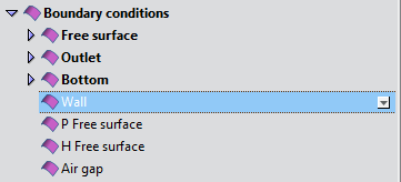
• Wall: Condition to be applied on fixed surfaces where waves will bounce back. This condition impose a no flow boundary condition for the total velocity potential. It can be applied on non-horizontal surfaces bounding the lower part of the computational domain to simulate irregular sea bottom (then the Bottom boundary condition should not be applied).

  

  Fig. 1.82 Wall interface

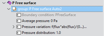
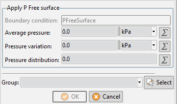
• PfreeSurface: Condition to be applied on free surfaces where pressure will be applied. Next figure shows an example of a PFreeSurface for a wave energy device based on the oscillating water column principle. This condition is to be applied on surfaces located at the plane z=0, and the Free Surface boundary condition have to be applied as well. On each node over the selected free surfaces, a specific pressure will be applied. 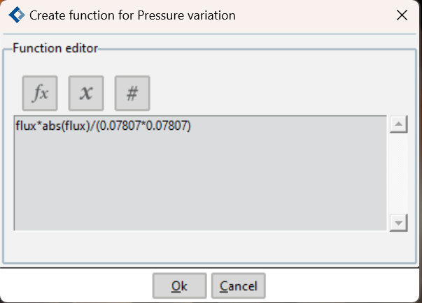This pressure is obtained as: \(P=(P_{average}+P_{variation}(t))·P_{distribution}(x,y)\), where P is the pressure to be applied, P_average is an average pressure constant in time and uniform in space, P_variation (t) is a time dependent pressure uniform in space, and P_distribution (x,y) is a pressure distribution in space and constant in time. The formulation for each component of the pressure is introduced via the function editor, whose variables are described in Appendix A.

  

  Fig. 1.83 P Free surface tree

  

  Fig. 1.84 P Free surface interface

  

  Fig. 1.85 P Free surface interface. Pressure variation.

  

  Fig. 1.86 P Free surface geometry

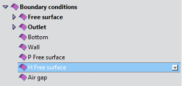
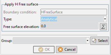
• HfreeSurface: Condition to be applied on specific free surfaces where the free surface elevation is limited in height (no higher than specified values). This condition is to be applied on surfaces located at the plane z=0, and the Free Surface boundary condition has to be applied as well. The limitation in height can be imposed in two different ways:

  • Analytical: the elevation limit is introduced via an analytical function using the function editor.

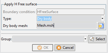
  • Dry body: the elevation limit is introduced via a three dimensional surface mesh. The vertical projection of this mesh should cover the portion of free surface where the HreeSurface boundary condition has been imposed. This mesh will move following the body movements, and pressure over the vetted portions will be calculated, as well as the resulting forces and moments. These forces and moments can be introduced into the body dynamics via the function editor provided in the external loads section.

  • Tcl script: The elevation limit is defined in a Tcl script. See Appendix B: Tcl extension section for further information.

  

  Fig. 1.87 H Free surface tree

  

  Fig. 1.88 H Free surface analytical

  

  Fig. 1.89 H Free surface dry body

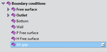
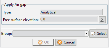
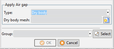
• Air gap: Condition to be applied on specific free surfaces where the free surface elevation is limited in height (no higher than specified values), and air gap results needs to be known. This condition is to be applied on surfaces located at the plane z=0, and the Free Surface boundary condition has to be applied as well. The limitation in height can be imposed in two different ways:

  • Analytical: the elevation limit is introduced via an analytical function using the function editor.

  • Dry body: the elevation limit is introduced via a three dimensional surface mesh. The vertical projection of this mesh should cover the portion of free surface where the Air gap boundary condition has been imposed. This mesh will move following the body movements, and air gap over the vetted portions will be calculated.

  

  Fig. 1.90 Air gap tree

  

  Fig. 1.91 Air gap analytical

  

  Fig. 1.92 Air gap dry body

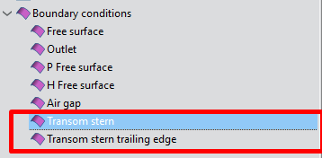
• Transom stern: when considering transom sterns, flow detachment happens at the lower edge of the transom. Since potential flow is incapable of predicting this sort of detachment, a transpiration model is used in SeaFEM to enforce it. To do so, the no flux body boundary condition is no longer applied to the body surfaces where the transom stern condition is applied. On the contrary, a flux is allowed on these surfaces.

• Transom stern trailing edge: this condition is used to enforce that the detachment edge belong to the free surface stream surface.

  

  Fig. 1.93 Transom stern and trailing edge. These conditions are available if Type of analysis >> Towing is activated.

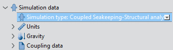
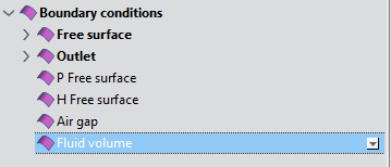
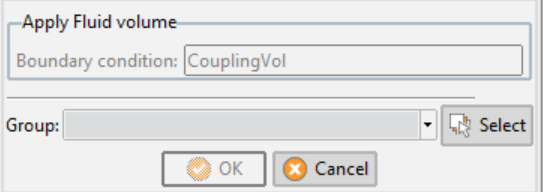
• Fluid volume: this condition is only available in Coupled Seakeeping-Structural analysis. For this kind of analysis, it is mandatory to apply this boundary condition to the entire volume defining the SeaFEM domain of analysis. Strictly speaking, this is not a boundary condition, but a property of the model that is necessary to identify the seakeeping domain and to differentiate it from the structural mesh.

  

  Fig. 1.94 Coupled Seakeeping - Structural analysis. In this case, it is necessary to select fluid volume.

  

  

  Fig. 1.95 Fluid volume interface.