Tdyn-tutorial4-two dimensional flow passing a cylinder
Problem description
The fourth tutorial analysis is a case of two-dimensional flow passing a cylinder in the low Reynolds number range.
We choose a Reynolds number of Re = 100, for which we expect a vortex street in the wake of the cylinder (the well known von Kármán vortex street).
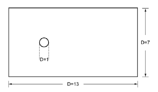
As in the two previous examples the geometry consists of a box that represents the control volume, which contains the body to be studied in this case a circular cylinder.
Geometrical description of the model
To automatically load the model simply left-click on the button below.
Introduction
The Reynolds number is calculated as in the cavity flow example. In this case the characteristic length of the problem is given by the diameter D of the cylinder. The complete set of parameters describing the problem are:
Parameter |
Symbol |
Value |
|---|---|---|
Characteristic length |
D |
\(1.0\ \text{m}\) |
Characteristic velocity |
v |
\(1.0\ \text{m/s}\) |
Fluid density |
\(\rho\) |
\(1.0\ \text{kg/m}^3\) |
Fluid viscosity |
\(\mu\) |
\(0.01\ \text{kg/m·s}\) |
which provide a Reynolds number \(Re = 100\)
Start data
For this case, the same kind of problems as in the previous tutorial must be loaded in the Start Data window of Tdyn.
2D Plane
Flow in fluids
See the Start Data section of the Cavity flow problem (Tutorial 1) or the Getting started manual for further details.
Pre-processing
Again the geometry for this example is created using the Preprocessor. First we have to create points with the coordinates given in the table below.
Nº |
X Coordinate |
Y Coordinate |
Z Coordinate |
|---|---|---|---|
1 |
-4.00 |
-3.50 |
0.00 |
2 |
-4.00 |
0.00 |
0.00 |
3 |
-4.00 |
3.50 |
0.00 |
4 |
9.00 |
3.50 |
0.00 |
5 |
9.00 |
0.00 |
0.00 |
6 |
9.00 |
-3.50 |
0.00 |
7 |
0.50 |
0.00 |
0.00 |
8 |
-0.50 |
0.00 |
0.00 |
The control volume will be generated by joining the created points using lines. Finally, the circle representing the cylinder’s section must be created using the Copy utility for copying the point while rotating it around a specified centre.
Utilities >> Copy
Such a copy option must be applied to point number 7 using the copy options shown in the figure below. This way, the point is going to rotate 180 degrees around the z-axis (by default if 2D is selected) about the center entered as first point. The option Do extrude: Lines traces the upper half of the circle.
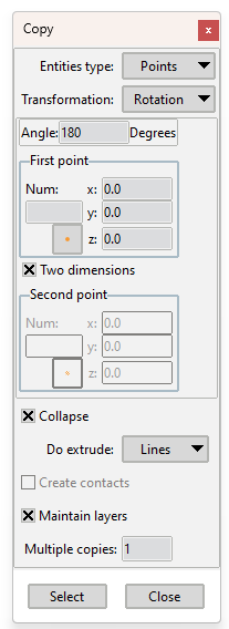
Copy dialog box
In order to draw the rest of the circle it is necessary to apply the same action to point No 8 just changing the value of the rotation angle to \(θ=-180\).
Materials
Physical properties of the materials involved in the problem are defined in the section following section of the Tdyn Data tree.
Materials and properties >> Physical Properties
Some predefined materials already exist, while new material properties can be also defined if needed.
For the present tutorial, only Fluid Flow properties are necessary for the fluid material which must be assigned to the only existing surface of the model (that defining the control volume of the present 2D case). This assignment is done using the following option.
Materials and properties >> Fluid
In this case, density and viscosity of the fluid are fixed to \(1.0\ \text{kg/m}^3\) and \(0.01\ \text{kg/m·s}\) respectively.
For every parameter, the respective units have to be verified, and changed if necessary (in our example, all the values are given in default units).
Initial data
Initial data for the analysis can be entered in the following section of the Tdyn data tree. In this case, only the Initial Velocity X Field must be fixed to \(1.0\ \text{m/s}\)
Conditions. & Initial Data >> Fluid Flow >> Initial and Field >> Velocity X Field
This initial data option will be further used in order to fix the velocity on the inlet edge of the control volume to the specified value.
Boundary conditions
Once the geometry of the control domain has been defined, we can proceed to set up the boundary conditions of the problem (access the conditions menu as shown in example 1). The conditions to be applied in this tutorial are:
a) Velocity Field [line]
Conditions & Initial Data >> Fluid Flow >> Velocity Field
This condition is used to fix the velocity on a line to the value given in the following section of the data tree.
Conditions & Initial Data >> Initial and Field Data
Velocity X Field and Velocity Y Field can define a space-time-variable dependant function and thus the Velocity Field condition can be used to specify a variable inflow. In order to do this, the corresponding Fix Field flag must be activated. It is also possible to fix the Velocity (during the run) to the initial value of the function given in the above mentioned entries. In order to do this, the corresponding Fix Initial flag should be marked.
Now, this condition will be assigned to the inflow and lateral lines of the channel (see figure below). In our case, all the velocity components have to be fixed for the inflow lines (i.e. mark Fix Field X and Fix Field Y) and only the vertical component for the lateral lines (i.e. mark Fix Field Y). Then, the corresponding components will be fixed to their initial values.
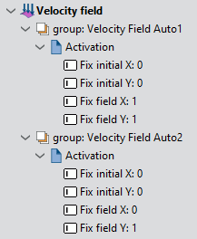
Velocity Field definition in Tdyn data tree.
b) Fix Pressure [line]
As mentioned in example 1, in order to solve the problem, the pressure must be fixed at least in one point of the control domain (taken as reference). Here we will apply the corresponding condition to the outflow lines of the domain.
Conditions & Initial Data >> Fluid Flow >> Fix Pressure
By imposing this condition, the value of the dynamic pressure defined in the corresponding Material (Fluid) (\(p = p_{o}-ρgz\) in our case) will be then assigned to this line.
Boundaries
a) Fluid Wall/Bodies
Conditions & Initial Data >> Fluid Flow >> Wall/Bodies
In this case only one Wall condition for the boundaries of the fluid domain is necessary. The V FixWall option will be chosen as the boundary type of the wall.
The condition has to be assigned to the lines that define the cylinder geometry.
Problem data
Other problem data must be entered by using the following options.
Fluid Dynamics & Multi-Physics Data >> Analysis
Fluid Dynamics & Multi-Physics Data >> Results
For this example, only the Fluid Flow must be solved by using the following parameters:
Analysis parameters
Number of steps : 1200
Time increment : 0.1 s
Max iterations : 3
Initial steps : 0
Output Step: 10
Output Start: 600
Remark: parameter OutPut Start is used to define when the program will begin to write the results. In this case, it has been fixed to 600 in order to reduce the size of the results file.
A brief summary of the boundary conditions, boundary definitions and material properties that have been applied to the control domain is given in what follows:
Condition |
Value |
Entity |
|---|---|---|
Velocity Field (line) |
Fix X Velocity, Fix Y Velocity |
Lines 4, 6 |
Velocity Field (line) |
Fix Y Velocity |
Lines 1,3 |
Fluid Wall/Bodies |
– |
Line 9, 10 |
Fluid |
– |
Surface 1, 2 |
Pressure Field (line) |
– |
Line 2, 7 |
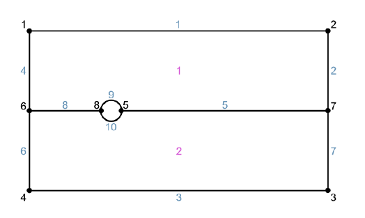
Boundary conditions applied to geometry
Mesh generation
As usual we will generate a 2D mesh by means of GiD’s meshing facilities.
Size assignment
The mesh should be finner in the vicinity of the cylinder. Therefore we will assign a size of 0.03 to the cylinder lines and points and a size of 0.1 to the symmetry line. The global size of the mesh is chosen to be 0.3, and an Unstructured size transition (Meshing Preferences window) of 0.5 will be used.
These values have been chosen by a ‘trial and error’-procedure, i.e. first some approximate values are chosen, out of experience and/or practical considerations. With these parameters a mesh is generated. If the obtained number of nodes is too large or too small, the parameters need to be adjusted correspondingly.
Finally, we will obtain an unstructured mesh consisting of 2160 nodes and 4464 triangle elements.
Calculate
The analysis process will be started from within GiD through the Calculate menu, as in the previous examples.
Post-processing
When the analysis is completed and the message Process ‘…’ started on … has finished. has been displayed, we can proceed to visualize the results by pressing Postprocess. For details on the result visualization not explained here, please refer to the Postprocessing chapter of the previous examples and to the Postprocessor user manual
The results shown below correspond to the last time step (t = 120 s) of the simulation.
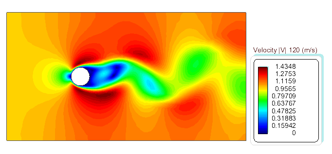
Contour fill of Velocity result
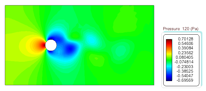
Contour fill of Pressure result
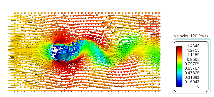
Vectors of Velocity result
The evolution in time of any parameter can be captured and visualized by means of the Animate utility of GiD (accessible through the Window main menu or by pressing Ctrl+m).
Selecting Save MPEG option in the Animate window allows to save the corresponding animation in MPEG format. In order to save disk space, it is advisable to reduce the GiD window size to the essential details, since the whole interior of the GiD main window will be saved. This can result in very large files. To prevent this, the empty space around the area of interest should be also minimized.
The following pictures show the time evolution of the fluid velocity at t=60 s, t=62 s, t=64 s, t=68 s, t=70 s, t=72 s, t=74 s, t=76 s and t=78 s.
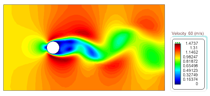
Contour fill of velocity at t=60 s.
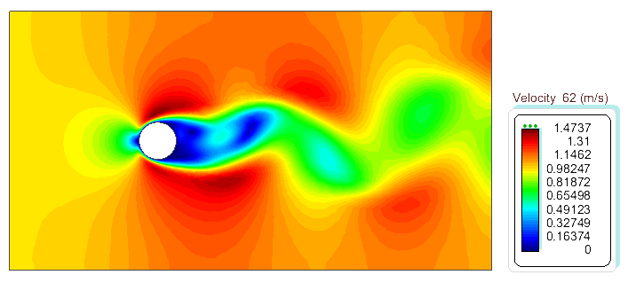
Contour fill of velocity at t=62 s.
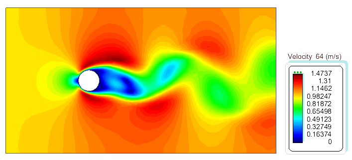
Contour fill of velocity at t=64 s.
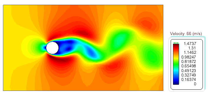
Contour fill of velocity at t=66 s.
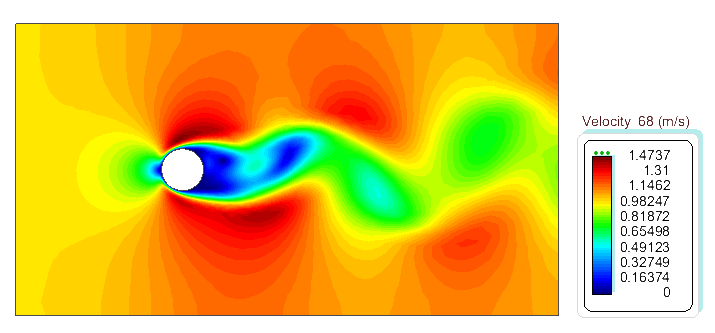
Contour fill of velocity at t=68 s.
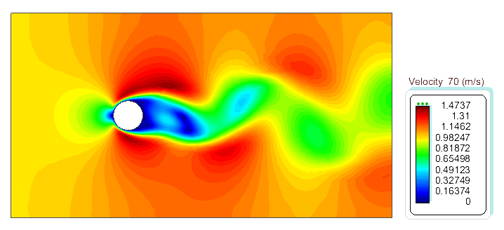
Contour fill of velocity at t=70 s.
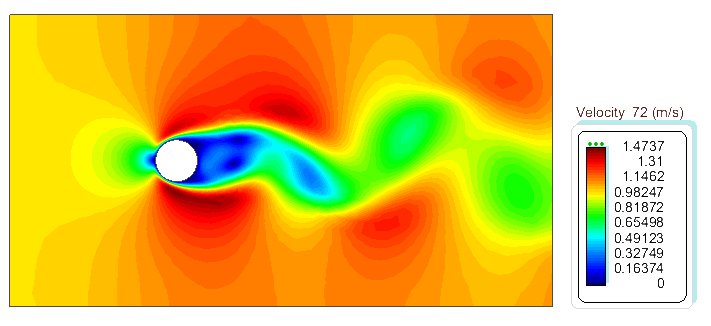
Contour fill of velocity at t=72 s.
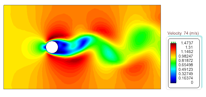
Contour fill of velocity at t=74 s.
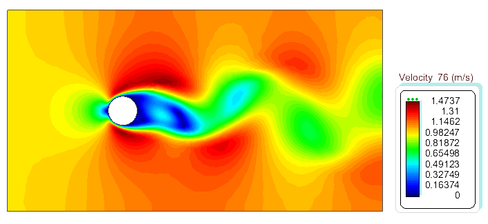
Contour fill of velocity at t=76 s.
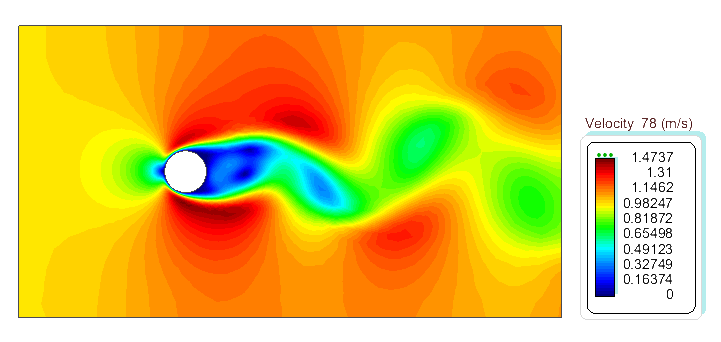
Contour fill of velocity at t=78 s.
Remarks
a) We can observe that the perturbances induced by the cylinder in the velocity and pressure fields reach the boundaries of the control volume. Normally this should be avoided by choosing a larger control volume, as the boundary conditions can perturb the solution. This has not been possible here because of the limits of the academic version of Tdyn (a larger domain would imply a larger mesh). Nevertheless quite accurate results are obtained.
b) The quality of the results can be verified by comparing the calculated period of the vortex shedding with experimental and other numerical results [12, 14]. The periodical character of the vortex shedding phenomenon is described by the Strouhal number, given by
\(Str=f·D/{v_\infty}\)
being
f the frequency of the vortex shedding
D the diameter of the cylinder
The computed period can be evaluated in many ways as for instance through the evolution of a variable at a point behind the cylinder, or through the evolution of the net force over it.
Here, we will first calculate the period using the graphical postprocessing capabilities of Tdyn.
First, load the Tdyn post-process by using the following option of the main menu: Postprocess >> Start
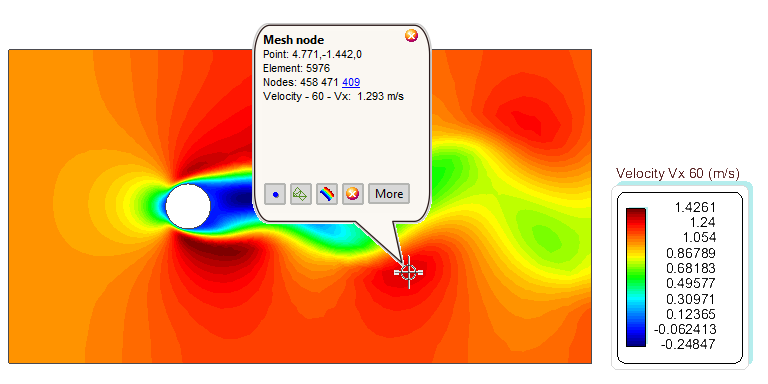
Once in the postprocess, select the physical result to be analyzed. In this tutorial, x-component of the velocity at a point downstream of the cylinder is selected. In a more central point, the x-component of the velocity would oscillate at twice the frequency, as it changes every time a vortex is shed. The lateral points, however, are only affected by vortices shed on the respective side of the cylinder. The point should also be far enough from the boundaries, as these can also affect the velocity evolution.
When left-clicking the point, a yellow information box is opened with information about the point coordinates and the result value at this point. Moreover, some buttons allow to get more information of this point. For instance, More button allows to open the Detailed information box.
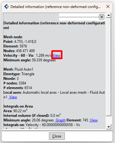
Detailed information box. The View link besides the result value opens a new dialog box with a time evolution graph of the shown result.
When the View link besides the result value (see the previous figure) is left-clicked, then a dialog box with a time evolution graph of the shown result is opened.
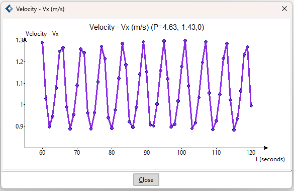
Time evolution graph of x-component velocity at the selected point.
As can be seen the resolution of the graph is not good enough since just one point is drawn every 10 time steps (every second) as it was indicated in the results output section of the data tree. However the period can be estimated quite accurately to be T = 6.0 s.