Tdyn-tutorial1-cavity flow

model case

Problem description

This example is the first of a series of tutorials intended to teach TDYN users all the capabilities the software provides for modelling multiphysics phenomena.

This first tutorial provides a concise guide on how to use TDYN to prepare a fluid dynamics simulation. Since this is the first example that a new TDYN’s user should read, all the steps necessary to prepare the simulation will be described in detail. In subsequent tutorials we will omit many of the basic steps described here, which are common to the setup process of any multiphysics simulation using TDYN. In these cases, references to the present tutorial will be included for further details.

For the present case, the geometry of the tutorial model can be extracted from the following link:

model geometry

The IGES file can be imported within TDYN using the following option of the main menu Files >> Import >> IGES

Hence, from now on, we will start every tutorial by importing the corresponding geometry as indicated above.

Alternatively, the model ready to be meshed and run can be downloaded from the following link:

Introduction

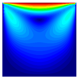
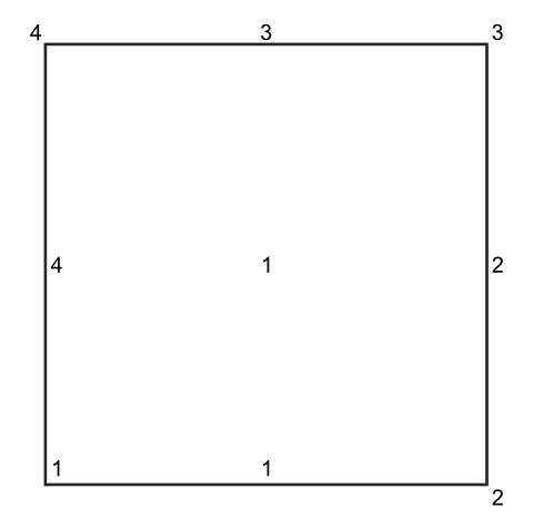
This example shows the necessary steps for studying the flow pattern that appears in a lateral, cavity of a by-flowing fluid one side of the cavity being swept by the outer flow. The flow pattern will be calculated using incompressible Navier-Stokes equations for a Reynolds number of 1. In order to capture turbulence effects that may appear at higher Reynolds numbers, a finer mesh would be necessary. The geometry of this problem simply consists of a square representing a cavity, its top face being swept by the passing fluid. This problem is a two-dimensional case solved to illustrate the basic capabilities of Tdyn.

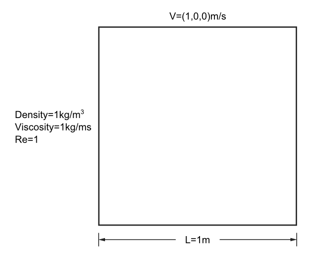
Schema of the 2D cavity flow problem

The Reynolds number is defined as \(Re = \rho \cdot V \cdot L / \mu\). In this equation, \(L\) represents the characteristic length of the problem, which in this case is the edge length of the cavity, \(\rho ` and :math:\)mu` are the density and the viscosity of the fluid respectively, and \(V\) is the velocity of the flow on the swept line. For the example to be solved here, we can choose arbitrarily:

Problem characteristics

• Characteristic length : \(L = 1.0 m\)

• Characteristic velocity : \(V = 1.0 m/s\)

• Fluid density : \(\rho = 1.0 kg/m^3\)

• Fluid viscosity : \(\mu = 1.0 kg/m\cdot s\)

By substituting these variables by their value in the equation above we obtain the Reynolds number \(Re = 1\).

Start data

The first step to prepare a simulation using TDYN is to select the type of analysis to be performed. This can be done within the Start Data window that appears by default the first time the user starts TDYN. If the window does not appear by default, you can open it using the menu option Data >> Start data

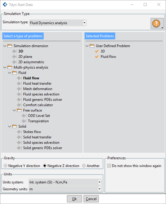
Start Data window as it is shown to the user the first time it starts TDYN

For further details on how to use the Start Data window and other important TDYN’s GUI tools, please refer to the ‘Getting started manual’ that can be accessed from the help icon at the top right corner of the Start Data window itself. For the present case, only the 2D plane and the flow in fluids capabilities of Tdyn are necessary. Hence, to setup the present simulation follow the steps below:

1. Open the Start Data window by using the menu option Data >> Start data

2. From the Start Data window, select the Fluid Dynamics analysis simulation type.

3. From the left panel of the Start Data window select the options 2D Plane and Fluid flow.

4. Press the Ok button to proceed to the working area of TDYN.

Note

Note that for 2D plane problems the active working plane is X-Y. Hence, for this type of analysis gravity vector must be directed along the Y axis since Z-axis is not available.

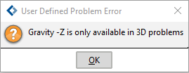
Warning message indicating that Z-axis is not available in “D plane problems and that gravity must be directed along the Y-axis.

Pre-processing

For this first tutorial and for the sake of exemplification, we will describe in detail how to create the geometry of the present case study. The geometry of this problem simply consists of a square representing a cavity, its top face being swept by the passing fluid. To create the box that encapsulates the flow, we only have to create the corresponding vertices, lines and surfaces using the Pre-processor tools. To do this, proceed as follows:

1. First, the points with the coordinates listed below must be created:

Point number	X coordinate	Y coordinate
1	0.000	0.000
2	1.000	0.000
3	1.000	1.000
4	0.000	1.000

To this aim, use the following main menu option Geometry >> Create >> point

Enter point coordinates in the command line located above the TDYN drawing area:

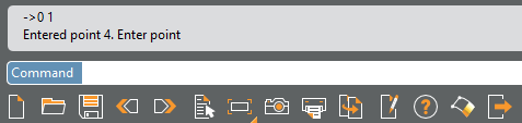
Command line located above the drawing central area of Tdyn where point coordinates must be introduced to generate the vertices of the cavity’s domain.

1. Then the lines have to be created joining the corresponding points. Use the following option (use Join or Ctrl+A to catch already existing points with the mouse button) Geometry >> Create >> Straight line and select the two points defining each line.

2. Once all the lines have been created, the surface that must represent the cavity (i.e. the control domain) has to be created by using Geometry >> Create NURBS surface >> By contour. Select the four lines that define the contour of the square domain.

Note

It is important to note here that the surface normals must be oriented in the OZ positive sense. This may be checked using the following option from the main menu View >> Normals >> Surfaces and selecting the surface or surfaces whose normals must be checked.

If you need to change the orientation of a normal, use the following menu sequence Utilities >> Swap Normals >> Surfaces and select the surface or surfaces whose normals are going to be swapped.

Materials

Physical properties of the materials used in the solution of the problem at hand can be specified in the following section of the Tdyn Data tree.

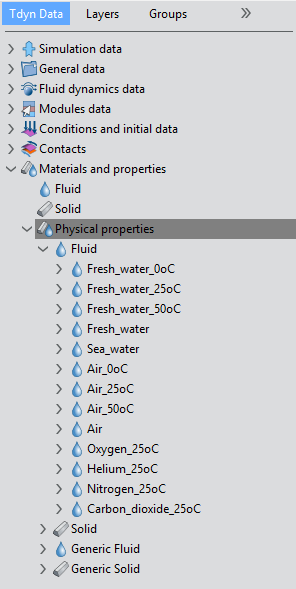
‘Physical properties’ section of the data tree where new materials can be created and the existing ones can be edited

If necessary, new materials can be created by right-clicking on any of the existing materials container in the data tree and selecting the option ‘Create new material’.

Materials and properties >> Physical properties >> Generic Fluid >> Create new material

Properties of the newly created material can be edited by double-clicking over the corresponding material label. By doing this, the following fluid flow dialog is open where fluid properties can be specified. In the present tutorial, density and viscosity of the fluid are fixed to 1 Kg/m3 and 1 Kg/mcdot s respectively. For every parameter, the corresponding units have to be verified, and changed if necessary (in our example, all the values are given in default units).

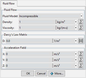
Fluid flow definition window where fluid material properties can be specified

Note that many of the options have specific on-line help that can be accessed by clicking on them with the right button of the mouse or by simply moving the mouse above the corresponding option. The defined material is finally assigned to the domain of analysis that in this case corresponds to the only existing surface in the model actually defining the cavity flow domain. To assign the fluid material proceed as follows:

1. Double-click over the following option of the data tree Materials and properties >> Fluid

2. The Apply Fluid dialog window will open. Within the Material drop-down list, select the material whose properties were previously defined.

3. Press the Select button and select with the cursor the squared-shape surface that defines the cavity.

4. In the Group entry of the Apply Fluid dialog window, enter the name you want to use to identify the group to which the material is being assigned.

5. Finally, press the Ok button to accept the material assignment and leave the dialog.

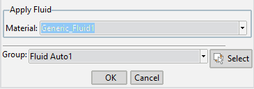
‘Apply Fluid’ dialog window where the fluid material must be selected and assigned to the corresponding geometry entities

Boundary conditions

Once we have defined the geometry and the material, it is necessary to set the boundary conditions of the problem. Boundary conditions, material properties and all the values of the various simulation parameters are specified and controlled in Tdyn by using the ‘Tdyn Data tree’. For further details on how to use the data tree, please refer to the ‘Getting started manual’ that can be accessed from the help icon at the top right corner of the ‘Start Data’ window. In this section we will describe in detail how to apply the boundary conditions of the problem. This is done in the ‘Conditions and initial data’ section of the ‘Tdyn Data tree’. The conditions to be specified in the present case study are the following ones: - Fix velocity at the swept edge of the cavity - Fix pressure at a reference point - A wall condition at the lateral and bottom edges of the cavity All three conditions and how to apply them are described in detail in what follows:

Fix Velocity [over a line]

Conditions and initial data >> Fluid flow >> Fix velocity

This condition is used to impose the velocity on a line. The fields in the values tab of the ‘Fix Velocity’ condition window store the velocity components (X and Y) given in global axes. The flags ‘Fix X Velocity’ and ‘Fix Y Velocity’ in the activation tab of the window allow to indicate if the corresponding components have to be fixed or not. If the corresponding ‘Fix’ flag is not selected, the corresponding values field will be disabled. In the present example this condition is going to be assigned to the line swept by the flow. In our case, the X-component of the velocity vector will be set to 1.0 m/s, and the Y-component to zero. Then, all the velocity components have to be fixed to the specified value (i.e. mark Fix X Velocity and Fix Y Velocity) as shown in the figure below.

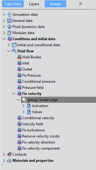
Fix velocity boundary condition selected in the Tdyn Data tree

To apply the boundary condition proceed as follows:

1. Double-click on the Fix Velocity option of the data tree Conditions and Initial Data >> Fluid Flow >> Fix Velocity

2. Check the options Fix X velocity and :guilabel:`Fix Y velocity`within the activation tab of the Fix Velocity condition.

3. Select the lines icon to indicate the type of geometrical entity to which the boundary condition will be applied

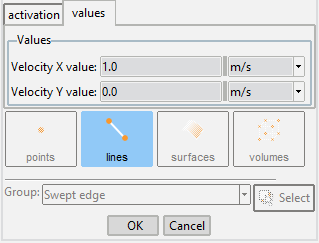
4. Enter the value 1.0 within the Velocity X value field of the values tab and the value 0.0 for the Velocity Y value component.

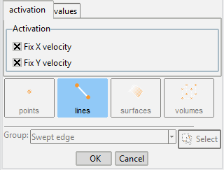
‘Activation’ window of the ‘Fix velocity’ boundary condition. In this case both, X and Y components of the velocity are enforced

align:

center

‘Values’ window of the ‘Fix velocity’ boundary condition. In this case the X component of the velocity is set to 1.0 m/s while the Y

1. Press the Select button and choose the top edge of the cavity where the ‘Fix velocity’ condition is going to be applied.

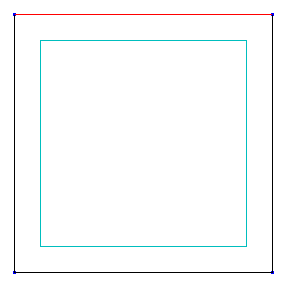
1. In the Group entry, enter the name you want to use to identify the applied boundary condition. In this example we use the name ‘Swept edge’.

2. Finally, press the Ok button to apply the condition and leave the dialog.

Fix Pressure [over a point]

Conditions and Initial Data >> Fluid Flow >> Fix Pressure

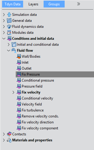
Fix Pressure boundary condition as it appears in the Tdyn Data tree

In most cases, it is recommended to fix the pressure at least in one point of the control domain (taken as reference). If this condition is not applied, Tdyn makes some corrections and the solution of the problem is equally achieved most of the times. In this case, the ‘Fix Pressure’ condition will be applied to the bottom left corner. To this aim, follow the following procedure:

1. Double-click on the Fix Pressure option of the data tree Conditions and Initial Data >> Fluid Flow >> Fix Pressure

2. Enter the value 0.0 within the Pressure value entry of the Edit Fix Pressure dialog window.

3. Select the points icon to indicate the type of geometrical entity to which the pressure boundary condition will be applied.

4. Press the Select button and choose the point at the bottom left corner of the cavity where the Fix Pressure condition is going to be applied.

5. In the Group entry, enter the name you want to use to identify the applied boundary condition. In this case we use the name Pressure ref point.

6. Finally, press the Ok button to apply the boundary condition and leave the dialog.

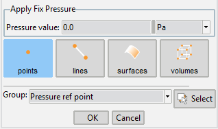
‘Apply Fix Pressure’ dialog window corresponding to the ‘Fix Pressure’ boundary condition. In this case the pressure at the left-bottom corner of the cavity domain is fixed to zero

Wall/Bodies boundary condition [over lines]

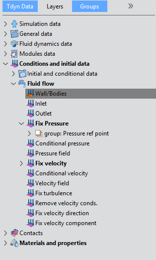
Wall/Body boundary condition as it appears in the Tdyn Data tree

Fluid wall and bodies are used to define fluid boundary properties in an automatic way. During the post-process, forces on fluid bodies can also be drawn. If necessary, new fluid boundaries can be created, based on the existing ones. In the present case, the wall body condition will be used to impose the natural null velocity condition at the boundaries of the cavity. To apply the condition, proceed as follows:

1. Double-click over the all/Bodies option of the data tree Conditions and Initial Data >> Fluid Flow >> Wall/Bodies

2. Since in the present case study we are dealing with a fluid domain, choose the option Fluid within the Fluid/Solid wall drop-down list of the Wall Type frame.

3. Choose the V FixWall option in the Boundary type drop-down list.

4. Press the Select button and choose the left, right and bottom edges of the cavity where the Wall/Body condition is going to be applied.

5. In the Group entry, enter the name you want to use to identify the applied boundary condition. In this case we use the name Cavity wall.

6. Finally, press the Ok button to apply the boundary condition and leave the dialog.

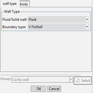
‘Wall type’ dialog window corresponding to the ‘Wall/Bodies’ boundary condition. In the present tutorial the ‘Wall/Bodies’ condition is applied to the lateral and bottom walls of the cavity and the natural null-velocity boundary condition is enforced by selecting the ‘V FixWall’ boundary type

Problem data

Once the boundary conditions and the materials have been assigned, we have to specify the remaining parameters of the simulation. Several data, as for instance the time increment for every time step and the type of problems to be solved, can be defined. The following are few of the most useful options (see Tdyn’s user and reference manual for further details):

• Number of steps: Number of steps of the simulation. Total time of the simulation will be (Number_of_Steps X Time_increment).

• Max. iterations: Maximum number of iterations of the non-linear fluid scheme (recommended values 1-3).

• Time increment: Time increment for each time step (recommended values < 0.1 * Length / Velocity).

• Output step: Each Output_Step time steps the results will be written.

• Output start: Results will be written after Output_Start time steps.

In this tutorial the analysis data must read as follows. Parameters not reported in this list should keep their default values.

Problem data

• Number of steps: 20

• Time increment: 0.1 s

• Max. iterations: 5

• Initial steps: 0

• Start-up control: None

• Restart: Off

• Processor unit: CPU

• Multiprocessor mode: Parallel

• Use Hypre Solvers: Off

• MPI: Off

• Steady state solver: Off

Within this section of the data tree, it is also possible to define solver properties (see ‘Fluid solver’ and ‘Solid solver’ blocks) symmetry planes (see the ‘Other’ block) or customize the output of results (see the ‘Results’ block of data). In any case, all these options will not be changed for the present tutorial as long as the default values are pertinent for this simple case.

A brief summary of the boundary conditions, boundary definitions and material properties that have been applied to the control domain are given in what follows:

Condition	Entity
Fix velocity	Line 3
Fluid wall	Lines 1,2,4
Fluid	Surface 1
Fix pressure	Point 1

Mesh generation

Mesh size assignment

The size of the elements generated is of critical importance. Too big elements can lead to bad quality results, whereas too small elements can dramatically increase the computational time without significant improvement of the quality of the results. In order to generate the mesh select the following option in the main menu. It can also be accessed through the (Ctrl+g) shortcut.

Mesh >> Generate mesh

You will then be asked for the global element size. In this case, a global element size about 0.035 was used so that the final mesh contains about the maximum number of nodes allowed by the limited version of Tdyn. The outcome is the unstructured mesh shown in the Figure below, consisting of 994 nodes and 1870 triangular elements.

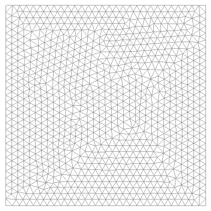
Finite element mesh consisting of 1870 triangular elements used for the present analysis of the cavity flow problem

Calculate

Once the geometry is created, the boundary conditions and materials are applied and the mesh has been generated, we can proceed to solve the problem. Through the ‘Calculate’ menu, we can start the solution process from within GiD. When pressing the Start button in the Calculate window, GiD will first write the calculation file called ProblemName.flavia (ProblemName being the name under which the problem has been saved in GiD), and then the process will start. Once the solution process is completed, we can visualize the results using the Post-processor module. The results file ProblemName.flavia.res will be loaded when selecting the Post-process option.

Post-processing

Once the message Process ‘…’ started on … has finished is displayed, we can visualize the final results by pressing Post-process (note that the problem must still be loaded; should this not be the case we first have to open the problem files again). Note that the intermediate results can be shown in any moment of the process, even if the calculations are not finished. The main post process window couples various sets of options, such as animations control, meshes, results or preferences selectors. In this way, each set of these options can be opened or minimized by pressing on its own grey rectangular button, which is located vertically at the left side of the post process window. For further details on postprocessing options see the Postprocess user manual

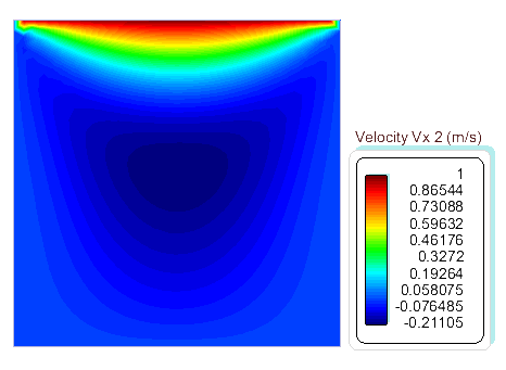
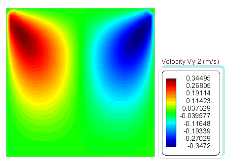
Results visualization

First we will visualize the velocity distribution on the surface domain by plotting the iso-contours of the x- and y velocity components.

The post-processing image can then be saved as a screen-shot of the current window by using the following option of the File menu:

Files >> Print to file

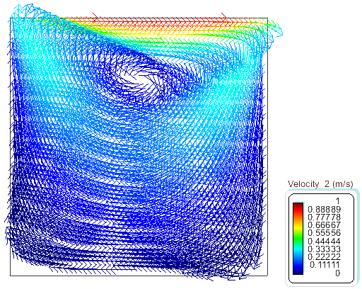
An overall impression of the flow pattern can be obtained by plotting the velocity vectors on the control surface.

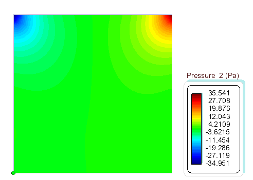
Finally, we can also plot the pressure distribution over the cut plane.

Graphs

As the graphs will be visualized over a cross section only, we have to proceed by cutting the mesh at the desired position. To do the cut, the following menu option must be applied

Postprocess >> Create cut plane

The cut plane will be perpendicular to the view drawn on the screen. In order to select the nodes of the mesh you can introduce points, either with the mouse or by introducing their co-ordinates manually in the Create cut plane/line window. In this example we will select a cut plane parallel to the original orientation of the control volume (XY-plane). In our case we used the points (0.0, 0.5) and (1.0, 0.5). By leaving only the cuts on we can plot and visualize the results over the cross section. Graphs can be easily drawn using the Line graph option of the contextual menu that can be accessed by right-clicking on the screen over the line cut. The currently selected result is plotted in the new graph. The resultant plot is shown in the following figure.

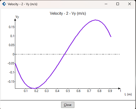
Line graph of Vy on the line of the cutting plane created above. The first point corresponds to x=1 and the last point corresponds to x=0.

For more details on the post-processing steps, please refer to the Pre/Post-processor user manual, or to the online help from the Help menu.