Tdyn-tutorial3-backward facing step
Problem description
This example is a two-dimensional study of a fluid flow within a channel with a backward-facing step. The flow pattern will be again calculated using the incompressible Navier-Stokes equations for a Reynolds number Re = 250, which for this problem lies in the laminar range (the transitional range lies between 1200 < Re < 6600).
The geometry basically consists on a box representing the channel with a step at the channel bottom.
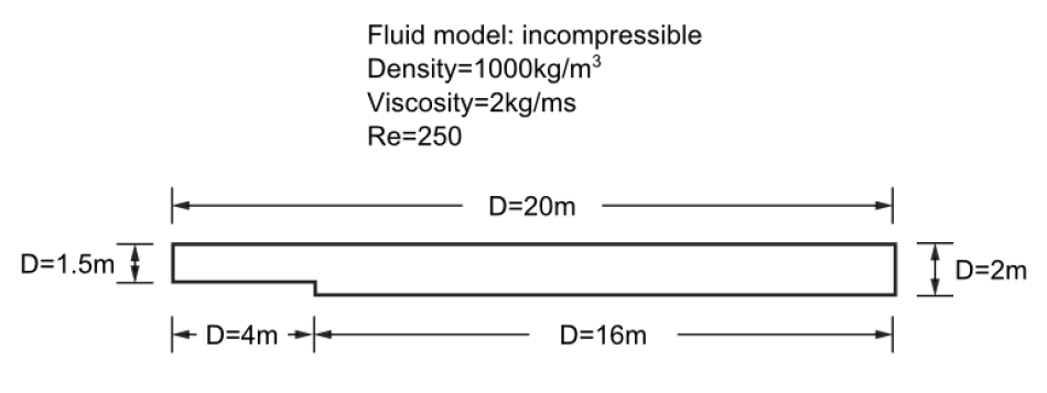
Geometrical description of the model
To automatically load the model simply left-click on the button below.
Introduction
The Reynolds number is defined here as: \(Re = 2v_{max}Dρ/3μ\) being the characteristic length D the height of the inlet channel.The factor 2/3 derives from the assumption of a parabolic velocity profile in the inlet section with vmax being the maximum velocity attained in this section. The value of the Reynolds number is obtained from the choice of the following parameters:
According to the equation presented above the following value is obtained for the Reynolds number :math: Re = 250
Start data
In this case, it is necessary to load the following types of problem in the Start Data window of the CompassFEM suite.
2D Plane
Flow in fluids
See the Start Data section of the Cavity flow problem (Tutorial 1) for details.
Pre-processing
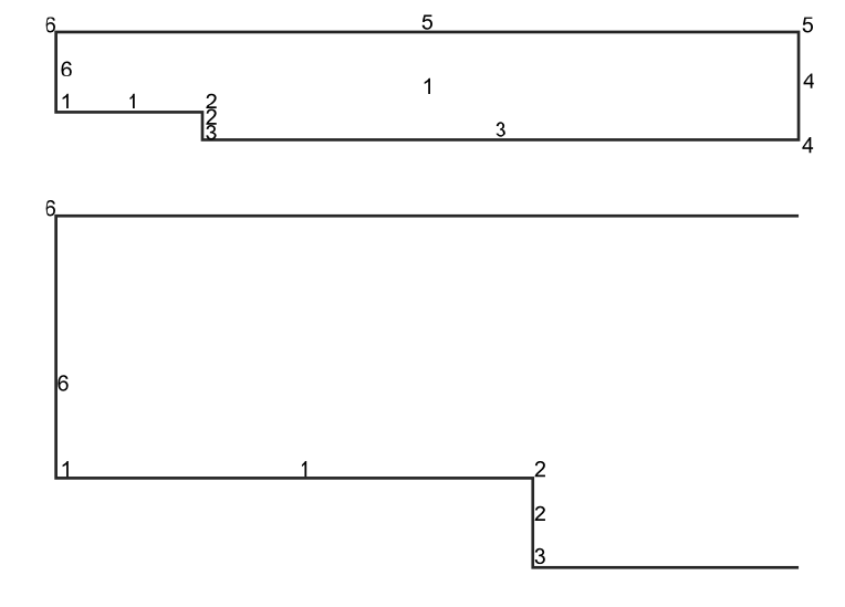
The geometry for this example will be created just as in the Cavity Flow tutorial using the Preprocessor module. The geometry will again resemble a box, but with a step at its bottom surface.
By entering the points with the co-ordinates given below, then joining them into lines and finally creating the control surface, we will obtain the geometry that can be checked in the Figure shown in the introduction section.
For details on creating the geometry, please refer to the Pre-processing section of Tutorial 1
Point number |
X Coordinate |
Y Coordinate |
|---|---|---|
1 |
0.0 |
0.5 |
2 |
4.0 |
0.5 |
3 |
4.0 |
0.0 |
4 |
20.0 |
0.0 |
5 |
20.0 |
2.0 |
6 |
0.0 |
2.0 |
Materials
Physical properties of the materials used in the problem are defined in the following section of the CompassFEM Data tree.
Materials >> Physical Properties
Some predefined materials already exist, while new material properties can be also defined if needed. In the present case, only Fluid Flow properties are necessary for the fluid material that has to be assigned to the only existing surface of the model (which defines the control volume of the present 2D case). This assignment is done through the following section of the data tree.
Materials >> Fluid
Different material assignements can be checked at any time by accessing the Draw groups options of the corresponding group within the section of the data tree.
In this case, Density and Viscosity of the fluid are fixed to \(1000.0 kg/m^3\) and \(2.0 kg/m·s\) respectively.
Initial data
The initial values of the velocity and other variables can be specified in the following section section of the Tdyn data tree.
Conditions & Initial Data >> Initial and Conditional Data >> Initial and Field Data
In the present case, a function that defines a parabolic profile must be inserted in the Velocity X Field:
Conditions & Initial Data >> Initial and Conditional Data >> Initial and Field Data >> Velocity X Field
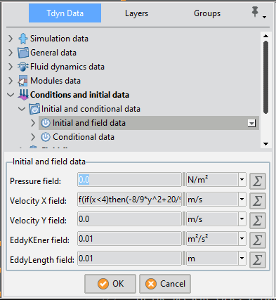
Conditions and Initial Data definition
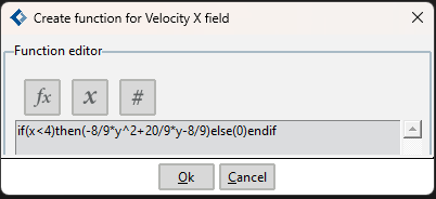
Velocity X field equation
Such a parabolic velocity profile must be applied at the inflow of the channel.
Boundary conditions
Once the geometry of the control domain has been defined, we can proceed to set up the boundary conditions of the problem. The conditions to be applied in this tutorial are:
Velocity Field [lines]
Fixed Velocity [lines]
Pressure Field [lines]
a) Velocity Field [lines]
This condition is used to impose the velocity on a line equal to the value given in the Initial and Field data section of the Tdyn data tree.
Any of the fields can be a time dependent function and in particular the Velocity Field condition can be used to specify a variable inflow. In order to do this, the corresponding Fix Field flags have to be marked in the dialog window that opens when double-clicking the following option of the data tree.
Conditions & Initial Data >> Fluid Flow >> Velocity Field
It is also possible to fix the Velocity (during the run) to the initial value of the function given in the corresponding Initial and Field data section. In order to do this, the corresponding Fix Initial flag should be marked in the dialog window mentioned above.
In this example the Fix Field X and Y conditions are going to be assigned to the inflow line of the channel. Coincidentally, this happens to be similar as the Fixed Velocity condition used in the cavity flow example; the difference here is that the fluid now enters through this surface, whereas in the previous case it was only tangent to the surface to which the condition was assigned.
Remark: the above condition will not work if the Start-up control option is activated in the Fluid Dyn. & Multiphy. Data- >Analysis section. Then this option must be switched off.
b) Fix Velocity [lines]
As explained in the example 1, this condition is used to impose the velocity on a line. For this example this condition is going to be assigned to the step line. Both velocity components will be set to 0.0 m/s. Then, all the velocity components have to be fixed to the specified value (i.e. Fix X Velocity and Fix Y Velocity must be activated).
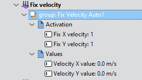
Fix velocity boundary condition
c) Pressure Field [line]
As explained in example 1, in order to solve the problem, the pressure must be fixed at least in one point of the control domain (taken as reference). Here we will apply the Pressure Field condition to the outflow line of the domain. The value of the dynamic pressure specified in the Initial and Field data section (\(p = p_{o}-ρgz\) in our case) will be further assigned to the outflow line. In this case, we will assume p = 0.
Boundary conditions
a) Fluid Wall/Bodies
In this tutorial, two different kind of boundaries will be applied to different parts of the model. Hence, two new wall conditions must be defined in the following section of the data tree, and they have to be further applied to the corresponding groups of entities in the model.
Conditions & Initial Data >> Fluid Flow >> Wall/Bodies
In this case the values of both fluid boundaries correspond to those of a V FixWall boundary type. The first one of the boundaries must be applied to the upper and bottom lines of the main channel, while the second one has to be assigned to the lines that define the step. Note that in the present case these boundaries could actually have been imposed by using only one boundary or by means of the line condition.
Conditions & Initial Data >> Fluid Flow >> Fix Velocity
However the above definition can be used for different problems.
Problem data
Other problem data must be entered in the section.
Fluid Dynamics & Multi-Physics Data >> Analysis
For this example, only the Fluid Flow must be solved by using the following parameters:
Analysis parameters
Number of steps : 300
Time increment : 0.5 s
Max iterations : 3
Initial steps : 25
Steady State solver: Off
A brief summary of the boundary conditions, boundary definitions and material properties that have been applied to the control domain is given in what follows:
Condition |
Value |
Entity |
|---|---|---|
Fix Velocity Line |
(0, 0) |
Line 2 |
Velocity Field Line |
if(x<4)then(-8/9*y^2+20/9*y-8/9)else(0)endif |
Line 6 |
Fluid Wall/Body 1 |
– |
Line 3,5 |
Fluid Wall/Body 2 |
– |
Line 1 |
Fluid |
– |
Surface 1 |
Pressure Field |
– |
Line 4 |
Relationship between boundary conditions and geometry
Mesh generation
The mesh will be generated automatically. We will generate a relatively coarse mesh, but it is chosen in order to minimize the number of nodes and to be able to calculate the case with the free version of Tdyn. In order to capture the flow pattern correctly, some critical areas need a finner mesh. Therefore, we will assign smaller mesh sizes to the areas of interest by means of the menu options
Mesh >> Unstructured >> Assign sizes on lines
Mesh >> Unstructured >> Assign sizes on points
In particular, we will assign the size 0.03 to the step line. The same element size will be assigned to the edge points of the step and a size of 0.06 to the inflow line. Finally, the Unstructured size transition will be set to 0.4 and the Elements general size to 0.2.
The outcome of the mesh generation process is the unstructured mesh shown below, consisting of almost 1700 nodes and 3000 elements.
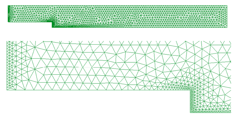
Mesh of the model
The number of mesh nodes and elements can be checked through the menu option
Utilities >> Status
If the size of the obtained mesh results to be significantly different from the size report herein, please make sure that the following option is set to None (especially if the nodes limit of Tdyn’s academic version is exceeded).
Utilities >> Preferences >> Meshing >> Automatic correct sizes
(Note that it is usually extremely convenient for beginners to activate the automatic correct sizes option).
Calculate
The calculation process will be started from GiD through the Calculate menu, exactly as described in the previous example.
The results file ProblemName.flavia.res is the file that will be loaded when pressing the Postprocess button.
Post-processing
When the calculations are finished, the message Process ‘…’, started on … has finished is displayed. Then we can proceed to visualizing the results by pressing the Postprocess button (therefore the problem must still be loaded; should this not be the case, we first have to open the problem file again).
As the post-processing options to be used are the same as in the previous tutorials, they will not be described in detail here again. For further information please refer to the Postprocessing chapter of Tutorial 1 and to the Pre/Postprocessor user manual or online help.
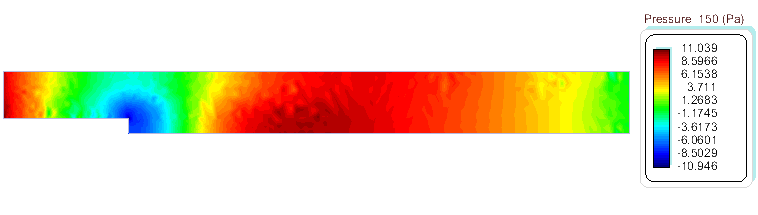
The results given below correspond to the last time step t=150 s.
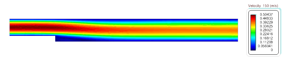
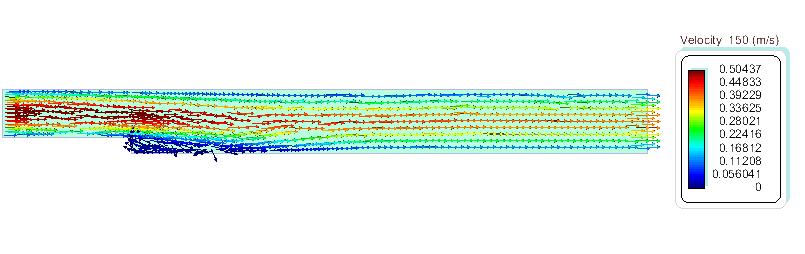
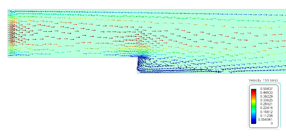
We can verify the numerical results by comparing them with experimental and other numerical results. At the low Reynolds number for which the present example is calculated, only the first vortex of the figure below will develop. Hence, the parameter that can be easily verified is the length x1. At \(Re = 250\) , the experimental values available for this parameter lie between \(x1 = 5.0 s - 6.0 s\) (being s the height of the step [1], while other numerical results available report \(x1 = 5.0 s\) [6,7].
The characteristic vortex length from the present simulation results to be \(x1 = 2.9 m\) that for the given height of the step \(s =0.5 m\) results in a value of the parameter \(x1 = 5.8 s\), which is a reasonably good result for the coarse mesh used.