Tdyn-tutorial2-cavity flow heat transfer
Problem description
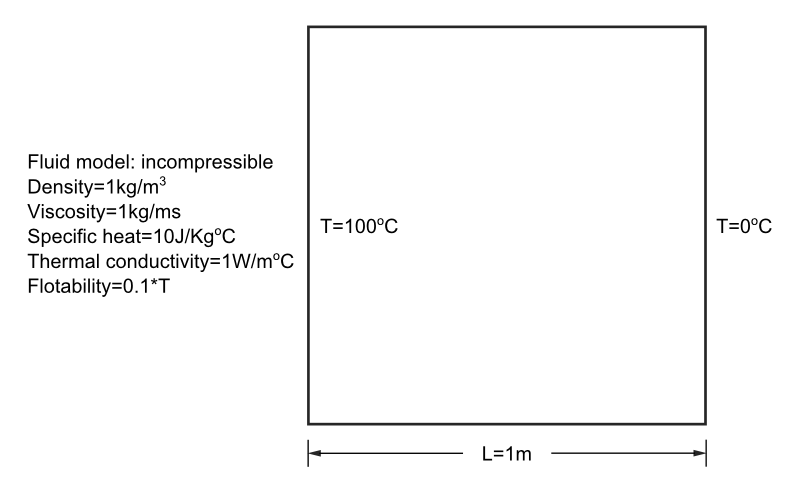
This example studies the flow pattern that appears in a square cavity when it is heated on one side. The flow pattern will be calculated using the incompressible Navier-Stokes equations coupled to the heat transfer equations by means of a floatability effect. Such an effect is controlled by the volume expansion coefficient property of the fluid so that the floatability is taken to be proportional to the temperature (in the present case floatability = \(0.1\cdot T\)). The geometry corresponding to this tutorial can be obtained in IGES format by right-clicking the following link:
The IGES file can be imported within TDYN using the following option of the main menu Files >> Import >> IGES
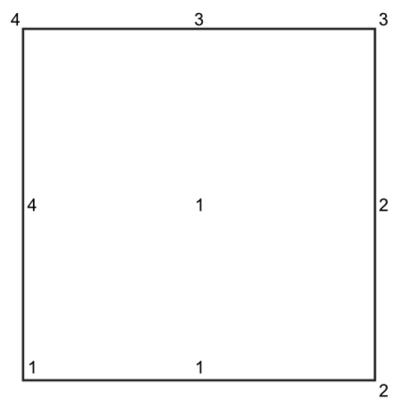
Description of the geometry of the model
Introduction
The fluid properties controlling the flow behavior are as follows:
Problem characteristics
Fluid density : \(\rho = 1.0 kg/m^3\)
Fluid viscosity : \(\mu = 1.0 kg/m\cdot s\)
Specific heat : \(c = 10.0 J/Kg \cdot Cº\)
Thermal conductivity : \(k = 10.0 W/m \cdot Cº\)
Start data
In this case, it is necessary to load the following types of problem in the Start Data window of TDYN.
2D Plane
Flow in Fluids
Heat transfer in fluids
See the Start Data section of the Cavity flow problem (Tutorial 1) or the Getting started manual for further details.
Pre-processing
The geometry simply consists of a square, representing a cavity. This problem is a two-dimensional case solved to illustrate the basic capabilities of the Fluid Dynamics and Multiphysics module of Tdyn.
The best way to proceed from example 1 is to save this file with a different name. This will preserve the geometry while deleting all the conditions of the problem.
Materials
Materials (Fluid)
In this example, fluid properties have to be fixed as follows:
Materials >> Physical Properties >> Generic Fluid >> Generic Fluid 1
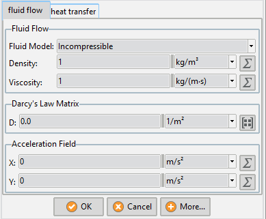
Fluid flow properties of a generic fluid
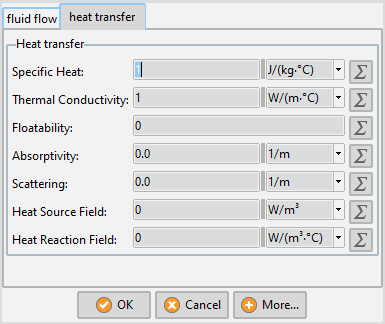
Fluid heat transfer properties of a generic fluid
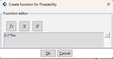
Fluid flotability function editor
Note that the Floatability field defines the coupling effect between fluid and thermal flow.
Materials are finally assigned to the only existing surface of the domain.
Materials >> Fluid >> Assign Fluid >> GenericFluid_1
Boundary conditions
Once we have defined the geometry of the control volume, it is necessary to set the corresponding boundary conditions. The only condition to specify here is a Fix Temperature condition along a line. For further details on how to assign boundary conditions, refer to the getting started tutorial of this manual.
Conditions & Initial Data >> Heat Transfer >> Fix Temperature
Fix Temperature [line]
The Fix Temperature [line] condition is used to fix the temperature on a line. In this example this condition will be assigned to the left line of the geometry with the value 100 ºC and to the right line with the value 0ºC.
Boundaries
Fluid Wall/Bodies
In this case a V FixWall boundary condition must be selected for the Fluid Wall definition (see figure below).
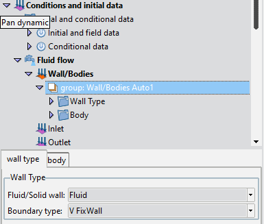
This property has to be assigned to all the contour lines of the geometry.
Problem data
Once the boundary conditions have been assigned, we have to specify the other parameters of the problem. These must be entered in the following section of the CompassFEM Data tree. In the present case the analysis data should be fixed as follows:
Fluid Dynamics & Multi-Physics Data >> Analysis
Analysis parameters
Number of steps : 100
Time increment : 0.1 s
Max iterations : 3
Initial steps : 0
Steady State solver: Off
A brief summary of the boundary conditions, boundary definitions and material properties that have been applied to the control domain is given in what follows:
Condition |
Value |
Entity |
|---|---|---|
Fix Temperature Line |
0 |
Line 2 |
Fix Temperature Line |
100 |
Line 4 |
Fluid Body |
– |
Line 1, 2, 3, 4 |
Fluid |
– |
Surface 1 |
Mesh generation
The mesh to be used in this example will be identical to that generated in example 1 (global element size 0.035).
Calculate
The calculation process will be started from within GiD through the Calculate menu, exactly as described in the previous example.
Post-processing
When the calculations are finished, a message Process’…’ started on … has finished is displayed. Then we can proceed to visualising the results by pressing Postprocess (therefore the problem must still be loaded; should this not be the case we first have to open the problem files again).
As the post-processing options to be used are the same as in the previous example, they will not be described in detail here again. For further information please refer to the Postprocessing chapter of previous example and to the Postprocessor user manual or online help. The results given below correspond to the last time step of t = 10s.
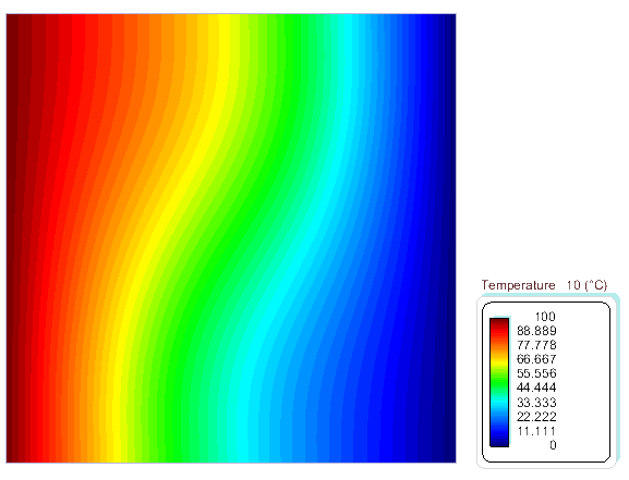
Thermal distribution
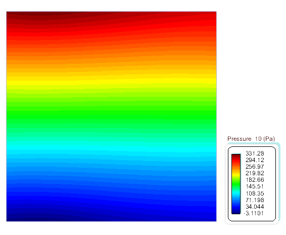
Pressure distribution
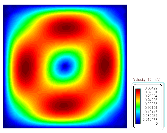
Velocity distribution
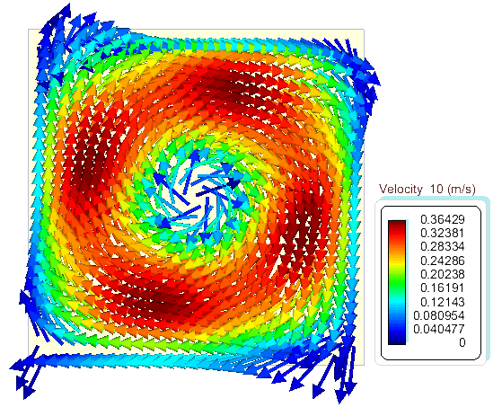
Velocity vector field distribution