2.1.3.2. Isotropic damage constitutive model

Table 2.2 Glossary

Symbol	Description	SI units
\(d\)	Damage parameter	–
\(\sigma\)	Uniaxial apparent stress	\(Pa\)
\(\bar{\sigma}\)	Uniaxial effective stress	\(Pa\)
\(E\)	Stiffness modulus	\(Pa\)
\(E^{sec}\)	Stiffness modulus	\(Pa\)
\(\Psi\)	Helmholtz free energy density	\(J/m^3\)
\(\Psi^e\)	Elastic strain energy	\(J/m^3\)
\(\varepsilon\)	Strain tensor	–
\(C^e\)	Undamaged elastic tensor	\(Pa\)
\(C^{sec}\)	Damaged secant stiffness tensor	\(Pa\)
\(\tau_{\sigma}\)	Stress energy norm	\(N^{1/2}/m\)
\(\tau_{\varepsilon}\)	Strain energy norm	\(N^{1/2}/m\)
\(F\)	Damage criterion in stress space	\(N^{1/2}/m\)
\(G\)	Damage criterion in strain space	\(N^{1/2}/m\)
\(r\)	Damage threshold internal variable	\(N^{1/2}/m\)
\(\dot{\xi}\)	Damage consistency parameter	\(N^{1/2}/m \cdot s\)
\(H\)	Softening/hardening modulus	\(N^{1/2}/m\)
\(r_0\)	Initial (undamaged material) damage threshold	\(N^{1/2}/m\)
\(H^d\)	Linear hardening/softening parameter	–
\(q_{\infty}\)	Saturation equivalent stress for exponential hardening law	\(N^{1/2}/m\)
\(A\)	Saturation equivalent stress for exponential hardening law	–
\(G_f\)	Fracture energy of the material	\(N/m\)
\(\tau_{\sigma}^I\)	Energy norm for symmetrical tension/compression damage model	\(N^{1/2}/m\)
\(\tau_{\sigma}^II\)	Energy norm for tension only damage model	\(N^{1/2}/m\)
\(\tau_{\sigma}^III\)	Energy norm for non-symmetrical damage model	\(N^{1/2}/m\)

The damage model implemented in RamSeries follows the isotropic damage model described in [Simo_1987], [Chaves_2003] and [Chaves_2013] which is based on the monotonic evolution (no healing effects) of the damage.

2.1.3.2.1. One-dimensional isotropic damage model

A simple 1D rheological model can be developed by considering that a material point is subjected to an apparent stress (\(\sigma\)) that acts on an apparent section (\(s\)), but due to the existence of micro-defects only the undamaged or effective section (\(\bar{s}\)) is sustaining the applied load, thus resulting in the existence of an effective stress (\(\bar{\sigma}\) ). Then, by considering the force balance, the following equilibrium equation is obtained:

(2.30)\[\begin{aligned} s \sigma = \bar{s} \bar{\sigma} \end{aligned}\]

Which can be rewritten as:

(2.31)\[\begin{aligned} \sigma = (1-s_d/s) \, \bar{\sigma} \equiv (1-d) \, \bar{\sigma} \end{aligned}\]

where \(s_d\) is the damaged section and the dimensionless ratio \(s_d/s\) represents the damage parameter denoted by \(d\), whose value must be within the range \(0 \leq d \leq 1\).

A simple constitutive equation to describe the one-dimensional isotropic damage model can be stated as follows:

(2.32)\[\begin{aligned} \sigma = E^{sec} \varepsilon \end{aligned}\]

Where

(2.33)\[\begin{aligned} E^{sec}= (1-d) E^e \end{aligned}\]

\(E^{sec}\) is the damage secant stiffness modulus. It can be observed from this relation that the damage variable can be interpreted as a measure of the loss of stiffness modulus of the material. The characteristic stress-strain behaviour of a material with isotropic damage is illustrated in Fig. 2.4 in the form of a uniaxial stress-strain curve.

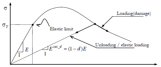
Fig. 2.4 One-dimensional stress strain curve characterizing the elastic-isotropic damage behaviour.

The energy equation of the system can be written as follows:

(2.34)\[\begin{aligned} \Psi = \frac{1}{2} \varepsilon \sigma = (1-d) \frac{1}{2} \varepsilon : E^e : \varepsilon = (1-d) \Psi^e \end{aligned}\]

where \(\Psi^e\) is the elastic strain energy.

2.1.3.2.2. Three-dimensional extension of the isotropic damage model

Note that the damage model described in the previous section depends on a single internal variable, namely the damage parameter \(d\). This implies that the degradation of the material is independent of the orientation so that the damaged elasticity tensor remains isotropic. To extend the isotropic damage model to the more general three-dimensional situation, let us generalize the expression of the Helmholtz free energy in Eq. (2.34) in the following form:

(2.35)\[\begin{aligned} \Psi = (1-d) \Psi^e = (1-d) \frac{1}{2} \varepsilon : \mathbb{C}^e : \varepsilon \end{aligned}\]

where the elastic strain energy \(\Psi^e\) is a function solely of the strain. \(\mathbb{C}\) is the elasticity tensor of the undamaged material. By thermodynamic considerations it can be demonstrated that the following expressions must hold:

(2.36)\[\begin{aligned} \sigma = \partial \Psi / \partial \varepsilon \end{aligned}\]

(2.37)\[\begin{aligned} \dot{d} \geq 0 \end{aligned}\]

By developing the rate of change of the Helmholtz free energy in Eq. (2.36), a constitutive equation suitable for the isotropic damage model can be obtained.

(2.38)\[\begin{aligned} \sigma = \frac{\partial \Psi}{\partial \varepsilon} = (1-d) \mathbb{C}^e : \varepsilon = (1-d) \bar{\sigma} \end{aligned}\]

Where \(\bar{\sigma}\) is the effective Cauchy stress tensor defined as:

(2.39)\[\begin{aligned} \bar{\sigma} = \mathbb{C}^e : \varepsilon \end{aligned}\]

From Eq. (2.40) it can be observed that, since the damage parameter is a scalar, the stiffness degradation is isotropic. The stress can be immediately computed once the strain (\(\varepsilon\)) and the damage internal variable (\(d\)) are known. And the constitutive equation can be interpreted as the sum of an elastic and an inelastic part.

(2.40)\[\begin{aligned} \sigma = (1-d) \mathbb{C}^e : \varepsilon = \mathbb{C}^e : \varepsilon - d \mathbb{C}^e : \varepsilon = \sigma^e - \sigma^i \end{aligned}\]

Finally, Eq. (2.33) that defines the one-dimensional damage secant stiffness modulus can be generalized to the three-dimensional case by defining the elastic-damage stiffness tensor in the following form:

(2.41)\[\begin{aligned} \mathbb{C}^{sec} = (1-d) \mathbb{C}^e \end{aligned}\]

Summarizing, the damage constitutive model is completely determined when de damage variable \(d\) is known at each time step of the loading/unloading process and when the constitutive equation is supplemented with a damage surface and a damage criterion plus a set of evolution laws for the internals variables and an energy norm of the stress (or strain) tensor. The various elements of the constitutive model listed here are briefly described in the following sections:

2.1.3.2.2.1. Energy norm in the stresses/strain space

A norm in the stress/strain space is a scalar measure that describes the stress/strain state at the current position of the material. Simple norms can be defined in terms of the equivalent stress (\(\tau_{\sigma}\)) and equivalent strain (\(\tau_{\varepsilon}\)) quantities defined as:

(2.42)\[\begin{aligned} \tau_{\sigma} = \sqrt{\sigma : (\mathbb{C}^e)^{-1} : \sigma} \end{aligned}\]

(2.43)\[\begin{aligned} \tau_{\varepsilon} = \sqrt{\varepsilon : \mathbb{C}^e : \varepsilon} \end{aligned}\]

(2.44)\[\begin{aligned} \tau_{\sigma} = (1-d) \tau_{\varepsilon} \end{aligned}\]

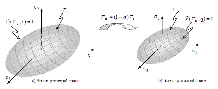
Fig. 2.5 Space norm representation.

2.1.3.2.2.2. Damage criterion

The damage criterion can be defined either in stress or strain space as follows:

(2.45)\[\begin{aligned} F(\tau_{\sigma},q) = \tau_{\sigma} - q(r) \leq 0 \end{aligned}\]

(2.46)\[\begin{aligned} G(\tau_{\varepsilon},r) = \tau_{\varepsilon} - r \leq 0 \end{aligned}\]

where \(r\) is an internal variable than can be interpreted as the current damage threshold and \(q\) is a function of \(r\) defining a hardening/softening variable. Both \(r\) and \(q\) are related to the damage variable \(d\). The damage criterion given by Eq. (2.45) implies that the stress state must be on or inside the damage surface. In the case of the stress state lying inside the damage surface, the material exhibits elastic behaviour either in a loading or unloading condition. On the contrary, in the case of the stress state lying on the damage surface, the material will behave elastically or continue increasing the damage depending on the actual loading condition.

From Eq. (2.46), it is observed that the undamaged material initial value (\(r_0\)) of the damage threshold determines the initial yield in the strain space so that the material starts fail when the strain energy norm exceeds the value \(r_0\). From an uniaxial test the value of \(r_0\) can be related to the yield stress (\(\sigma_y\)) measured in the laboratory:

(2.47)\[\begin{aligned} r_0 = \frac{\sigma_y}{\sqrt{E}} \end{aligned}\]

2.1.3.2.2.3. Evolution law

The evolution laws for the yield limit (\(r\)) and for the damage variable (\(d\)) are:

(2.48)\[\begin{aligned} \dot{r} = \dot{\zeta} (\varepsilon,r) \end{aligned}\]

(2.49)\[\begin{aligned} \dot{d} = \dot{\zeta} H(\tau_{\varepsilon},d) \end{aligned}\]

Where \(\dot{\zeta}\) is the damage consistency parameter and \(H\) is the continuum softening/hardening modulus.

2.1.3.2.2.4. Linear hardening/softening law

For the linear hardening/softening law it is assumed that \(q\) has the following linear relation with \(r\):

(2.50)\[\begin{split}\begin{aligned} q(r)=\begin{cases} r_0, & \text{if $r\leq0$}.\\ r_0 + H^d (r-r_0) \not < 0, & \text{if $r>r_0$}. \end{cases} \end{aligned}\end{split}\]

So that the hardening law is fully characterized by the value of the initial damage threshold \(r_0\) and the value of the hardening (softening) parameter \(H^d\) that, as shown in Fig. 2.6 , corresponds to the slope of the linear hardening/softening relation. As expected, positive values of \(H^d\) correspond to hardening behaviour while negative values correspond to softening.

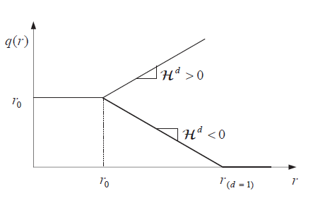
Fig. 2.6 Representation of the damage threshold using a linear law.

2.1.3.2.2.5. Exponential hardening/softening law

In the case of an exponential hardening/softening law (depicted in Fig. 2.7), the relation of \(q\) with \(r\) can be expressed as follows:

(2.51)\[\begin{aligned} q(r) = q_{\infty} - (q_{\infty} - r_0) \cdot e^{A(1-\frac{r}{r_0})} \end{aligned}\]

The hardening law is again fully characterized by two scalar values, the saturation equivalent stress \(q_{\infty}\) and the exponential factor \(A\) which is related to the fracture energy \(G_f\) of the material and the characteristic length of the element \(l_c\) by the following expression [Oliver_1990]:

(2.52)\[\begin{aligned} A=\left(\frac{g_f}{r_0^2}-\frac{1}{2}\right)^{-1} \end{aligned}\]

(2.53)\[\begin{aligned} g_f=\frac{G_f}{l_c} \end{aligned}\]

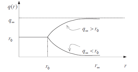
Fig. 2.7 Representation of the damage threshold using an exponential law.

2.1.3.2.3. Energy norms

The actual behaviour of the damaged material is strongly influenced by the yield damage surface but also by the actual energy norm under consideration. Three different energy norms are implemented in RamSeries, which are commonly used together with the isotropic damage model.These are briefly described in what follows.

2.1.3.2.3.1. Symmetrical tension-compression damage model (mode I)

This model can be used when the material behaves the same under tension or compression. In this case the energy norm can be expressed as:

(2.54)\[\begin{aligned} \tau_{\sigma}^I = \sqrt{\sigma : (\mathbb{C}^e)^{-1} : \sigma} = \sqrt{\bar{\sigma} : \varepsilon} \end{aligned}\]

For the sake of illustration, it is useful to consider a plane stress condition, in which case the damage surface is represented by an ellipse. By considering the mode I energy norm, we are assuming the stress limit \(\sigma_y\) to be the same in tension and compression. Additionally, the damage surface is assumed to evolve symmetrically as shown in figure Fig. 2.8.

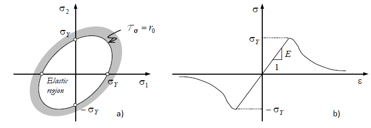
Fig. 2.8 Schematic representation of damage model’s Mode I energy norm. (a) Damage surface corresponding to a plane stress condition. (b) Uniaxial stress-strain curve in tension and compression.

2.1.3.2.3.2. Tension-only damage model (mode II)

In this model, damage is assumed to occur only in tension. Under compression, the material will always behave elastically and will never fail. In this case, the energy norm can be defined as:

(2.55)\[\begin{aligned} \tau_{\sigma}^{II} = \sqrt{\sigma^+ : (\mathbb{C}^e)^{-1} : \sigma} \end{aligned}\]

(2.56)\[\begin{aligned} \sigma^+ = \frac{\sigma + |\sigma|}{2} \end{aligned}\]

The relationship between real and effective stress still holds:

(2.57)\[\begin{aligned} \sigma^+ = (1-d) \cdot \bar{\sigma}^+ \end{aligned}\]

As in the previous section, it is useful to represent the Mode II damage surface corresponding to a plane stress condition and the uniaxial stress-strain curve for the corresponding material, in Fig. 2.9.

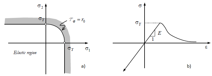
Fig. 2.9 Schematic representation of damage model’s Mode II energy norm. (a) Damage surface corresponding to a plane stress condition. (b) Uniaxial stress-strain curve in tension and compression.

2.1.3.2.3.3. Non-symmetrical damage model (mode III)

Finally, mode III energy norm can be used to simulate the mechanical response of materials whose behaviour under tension differs from that in compression. A typical application of this kind of energy norm is to model materials like concrete which exhibit quite larger strength in compression than in tension. The following energy norm can be used in these cases:

(2.58)\[\begin{aligned} \tau_{\sigma}^{III} = \left( \theta + \frac{1-\theta}{n} \right) \sqrt{\sigma : (\mathbb{C}^e)^{-1} : \sigma} \end{aligned}\]

Where \(\theta\) is a weight factor that depends on the actual stress state as follows:

(2.59)\[\begin{aligned} \theta = \frac{\sum\limits_{i=1}^3{\langle \sigma_i \rangle} }{\sum\limits_{i=1}^3{|\sigma_i|}} \end{aligned}\]

The parameter \(n\) is defined as the ratio between the compression and the traction elastic limits:

(2.60)\[\begin{aligned} n=\frac{\sigma_y^c}{\sigma_y^t} \end{aligned}\]

The Macaulay bracket \(\langle \sigma_i \rangle\) in the above expression is defined as:

(2.61)\[\begin{aligned} \langle \sigma_i \rangle = \frac{\sigma_i + | \sigma_i |}{2} \end{aligned}\]

The schematic representation of Mode III damage model is shown in figure Fig. 2.10.

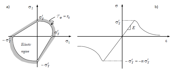
Fig. 2.10 Schematic representation of damage model’s Mode III energy norm. (a) Damage surface corresponding to a plane stress condition. (b) Uniaxial stress-strain curve in tension and compression.