RamSeries-Tutorial 2: Analysis of a shell structure

Model case

Model geometry

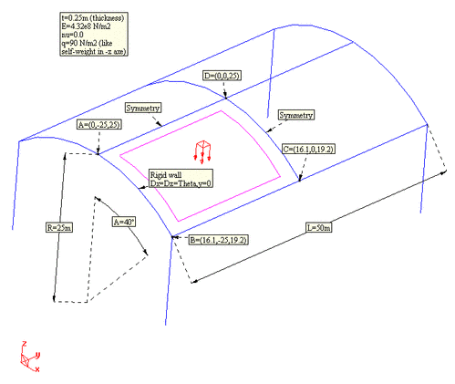
Schematic representation of the problem under analysis. Only one fourth of the entire structure is actually modelled taking advantage of the double symmetry resulting from the actual configuration of the problem.

Problem description

This tutorial aims to demonstrate the use of RamSeries capabilities for modelling shell structures. In particular, this model describes the analysis of a curved roof taking advantage of the double symmetry of the actual problem configuration. A sketch of the whole problem is shown in the figure below. One fourth of the total shell structure and the corresponding symmetry conditions are indicated to illustrate the actual problem being solved.

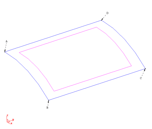
The geometry can be constructed in GiD using the following useful pre-processing commands which are described in detail in the GiD User’s Manual.

Geometry >> Create >> Line Geometry >> Create >> Arc Utilities >> Copy >> Rotate >> Do extrude lines Geometry >> Create >> NURBS surface >> By contour

The final model will be composed of 1 surface, 4 lines and all of its connecting points. Be careful to position the structure related to the global axes as seen in the figure to make it easier to follow the set up of the example as explained in the remaining part of the tutorial. The coordinates of the four vertices of the shell under analysis are reported in the following table:

Point number	X coordinate	Y coordinate	Z coordinate
Point A	0.000	-25.0	25.0
Point B	16.07	-25.0	19.15
Point C	16.07	0.0	19.15
Point D	0.000	0.0	25.0

Problem specification

To load the RamSeries type of analysis, choose the following option in the Start Data window:

Simulation type >> Structural analysis

The same option can be alternatively activated through the data tree by using the following option:

Simulation data >> Simulation type >> Structural analysis

The kind of problem under consideration in this tutorial, requires the following basic options to be selected:

• Simulation dimension: 3D

• Structural analysis element types: Shells

• Analysis type: Static analysis

• Material constitutive model: Linear-elastic model

• Geometrical constitutive model: Linear geometry

This setup can be configured from the Start Data window as explained in detail in the ::ref::Tutorial 1 - Analysis of a beam structure tutorial. Alternatively, all these options can be modified in the data tree if necessary.

Constraints

Constraints for shells can be either applied to points or lines. In this example, fixed constraints are applied to 3 boundary edges of the shell by using the following option of the data tree:

Constraints >> Fixed constraints

In particular, a condition resembling a rigid wall is applied to the edge AB. To this aim, X and Z displacements must be restrained as well as the rotation about Y global axis. Hence, the degrees of freedom are activated as indicated in the following table (non-activated degrees of freedom remain free) and the corresponding displacements are fixed to zero:

Activation		Values
X constraint	1	X value	0.0
Y constraint	0	Y value	0.0
Z constraint	1	Z value	0.0
Rot X constr	0	X value	0.0
Rot Y constr	1	Y value	0.0
Rot Z constr	0	Z value	0.0

On the other hand, lines CD and DA must have symmetry conditions. To this aim, degrees of freedom must be prescribed as shown in the following tables for CD and DA edges respectively:

Activation		Values
X constraint	0	X value	0.0
Y constraint	1	Y value	0.0
Z constraint	0	Z value	0.0
Rot X constr	1	X value	0.0
Rot Y constr	0	Y value	0.0
Rot Z constr	1	Z value	0.0

Activation		Values
X constraint	1	X value	0.0
Y constraint	0	Y value	0.0
Z constraint	0	Z value	0.0
Rot X constr	0	X value	0.0
Rot Y constr	1	Y value	0.0
Rot Z constr	1	Z value	0.0

Finally, edge BC remains completely free. In all these cases, the degrees of freedom refer to the global system axes.

Shell material properties

The shell under analysis in this tutorial is considered to be isotropic. To assign the section and material properties of an isotropic shell, use the following option of the data tree and setup the corresponding properties as shown below:

Materials and properties >> Shells >> Isotropic shells

• \(t = 250 \ mm\) (thickness)

• \(E = 4.32e8 \ N/m^2\) (Young modulus)

• \(\nu = 0.0\) (Poisson coefficient)

• \(\rho = 0.0 \ N/m^3\) (the self-weight of the shell is not considered)

Note: Remember that for an isotropic material: \(G=E/(2·(1+\nu))\) In this case \(G=E/2\)

Note also that the default local axes system is used. Following the axes criteria explained in detail in the RamSeries’ users manual, \(X'\) local axis will point towards the positive global \(X\) axis. \(Z'\) axis will be normal to the elements and \(Y'\) will be contained in the plane \(XZ\). Once the shell material properties are filled in, the condition must be assigned to the surface that defines the shell. Assigned conditions can be viewed at any moment by right-clicking on the created group and using the following option from the contextual menu:

Draw >> Draw values/groups/symbols

Load conditions

The load condition of the structure under analysis in this problem consists on a distributed load of \(90 N/m2\) directed to the negative direction of the global \(Z\) axis. Hence, a pressure load condition can be applied by using the following option of the data tree:

Loadcases >> Loadcase 1 >> Shells >> Pressure load

Factor	1.0
Loadtype	Global
X pressure	0.0 \(N/m2\)
Y pressure	0.0 \(N/m2\)
Z pressure	-90.0 \(N/m2\)

The resulting condition must be assigned to the surface that defines the shell under analysis.

Mesh generation

RamSeries can generate both, 3-node and 6-node triangular meshes. hence, it is possible to mesh the surface of the shell under analysis with either linear or quadratic triangles. The use of linear or quadratic elements can be controlled by using the following main menu option:

Mesh >> Quadratic type >> Normal | Quadratic | Quadratic 9

Note that the Quadratic9 option only applies to quadrilateral elements for which an extra node is located at the center of the element.

Note also, that in the structural analysis data tree an option exists to control the type of triangular element being used internally by the structural solver:

General data >> Analysis >> Element types >> Internal triangular element

This option is set by default to DKT. Nevertheless, a 6-node option is also available in which case 3-node triangular meshes are internally converted to 6-node meshes. Finally, a third option exists that allows to use an improved Drill-rotation triangular element.

As usual, the more elements are used to mesh the geometry, better accuracy in the results will be obtained. In change, larger computer times and RAM memory resources will be needed. The following option can be used at the end of the calculation to get information on the memory and computer time requirements:

Calculate >> View time table

It is usually convenient to mesh using smaller elements in those zones of the shell where larger result’s gradients are anticipated to exist. Mesh element sizes can be controlled using the following options to assign mesh sizes to the various geometrical entities (points lines surfaces and volumes) of the model.

Meshing >> Assign unstructured sizes >> Points Meshing >> Assign unstructured sizes >> Lines Meshing >> Assign unstructured sizes >> By chordal error

In this model, a default size of 1 is chosen to generate triangular meshes. To actually generate the mesh using such a default mesh size, use the following main menu option indicating the maximum element size allowed:

Meshing >> Generate >> 1

The resulting mesh contains will contain approximately 642 nodes and 1146 linear triangular elements. To get an insight on the precision of the results related to the number of nodes in the mesh, please take a look at the benchmark graphics provided in the appendix .

Calculate

If the model has not been saved yet, use:

File >> Save

and give a name to the model. To begin the analysis choose:

Calculate >> Calculate

The analysis runs as a separate process. Then, it is possible to continue working with GiD or exit the program. When the analysis is finished, a window will appear notifying it. If it has not run successfully, one window showing some error info will be supplied. Correct the error and run again. It is possible to visualize, when the process is running, some information about its evolution. Press:

Calculate >> View process info

One of the most important information that can be obtained in this window is the amount of RAM memory, expressed in Megabytes, needed by the solver. The total amount of memory required by the analysis code is somewhat bigger. For skyline solver, the total amount is about 10% more. For Sparse solver, it is about the double of memory. This data gives an idea of the maximum problem that can be solved in a given computer.

Postprocess and results analysis

The part of the program dedicated to visualize the results of the analysis is called Post-process. Once the calculation is finished, to enter in the post-process part and load automatically the results select:

Postprocess >> Start

To perform the operation correctly, it is necessary to have the model loaded inside the pre-processing part before going to post-process.

Visualization of local axes

The first important checking that must be done is to see if the local axes for every shell element are equal to the ones supposed when assigning the properties. Choose:

Postprocess panel >> Results >> Static >> Shells >> Local axes >> Local axes

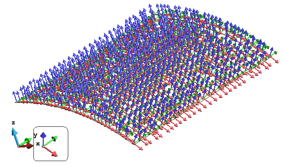
Local \(X'\) axis is drawn in color red, \(Y'\) axis in green and \(Z'\) axis in blue. If they are different than supposed, go to the pre-processing part, change the properties accordingly and calculate again.

It is possible to enter a different factor to change the display size of the axes. Just enter the new factor in:

Postprocess panel >> Preferences >> Vectors & Local axes >> Factor

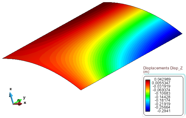
Deformation results

To visualize the deformed (with displacements contour fill on it) of the structure, select the following option and visualization preferences in the postprocess panel:

Postprocess panel >> Results >> Static >> Displacements >> Contour fill

Postprocess panel >> Preferences >> Deformed >> Draw: [Yes]

Postprocess panel >> Preferences >> Deformed >> Factor: [10]

Postprocess panel >> Preferences >> Deformed >> Result: [“Static displacements”]

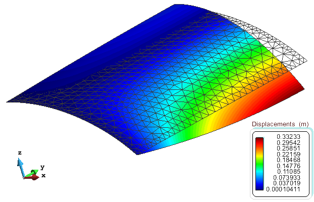
The deformation of the structure is drawn magnified in the screen in accordance to the deformation factor provided in the postprocess preferences panel. The magnification factor is automatically calculated if the “Adimensional factor” option is selected instead of providing a fixed factor. The deformation and the original configuration of the structure can be drawn together for the sake of reference. To this aim, select the following option if the preferences section of the postprocess panel:

Postprocess panel >> Preferences >> Deformed >> Draw original

Another way to see the magnitude of the deformation of the shell is to use:

Postprocess panel >> Results >> Static >> Displacements >> Disp. Z >> Contour fill

To see the numerical values of the deformation choose at any point, node or element:

Postprocess >> Mesh information

Try also pressing mouse left button over any structure element in the screen. Make the appropriate zooms to visualize properly the values.

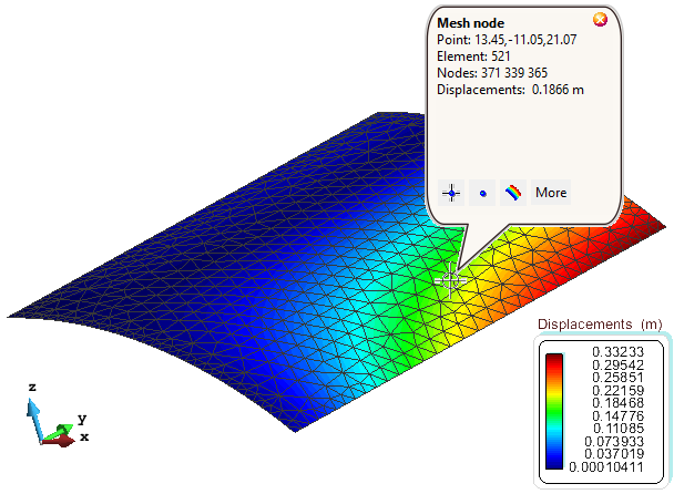
To switch off the labels press:

Mouse right button >> Label >> Off

In order to choose the visualization style for the shell, try:

Postprocess panel >> Meshes >> Display style

It is quite usual that there are local concentrations of strengths near the constraint points or near the nodal forces. In these cases, the scale of color has not enough contrast in the rest of the shell. To avoid it, it is possible to change the limits of the values of the contour fill. The zones of the shell that have values higher that the maximum limit or lower that the minimum one, will appear either black, transparent or in a defined colour, depending on the user preferences.

To define the maximum and minimum limits activate the corresponding checkbox, and define the limits:

Postprocess panel >> Results >> Limits

Right-click over the “Limits” label, leads to the following available options:

• Recalculate limits.

• Recalculate limits-all steps (only dynamic cases).

• Multiple results.

• Only active meshes.

• Legend colours.

• Redraw.

Strength results

All the strengths are reported referred to the local axes system of every shell (except the strengths in main axes). The visualization will be generally with a Contour Fill of every component of the strength although there are other ways to visualize them. To see the numerical value of the strength that is being visualized, choose:

Mouse right button >> Label >> All

Mouse right button >> Label >> Off

Both commands can be found in the menu that appears when pressing the secondary mouse button over the screen.

The strengths are the following:

Name		Default units	Remarks
Axial force	\(N_{x'} N_{y'} N_{x'y'}\)	\(N/m\)	Axial force in all the shell thickness per unit width of the shell
Momentum	\(N_{x'} N_{y'} N_{x'y'}\)	\(N·m/m\)	Momentum per unit width of the shell
Shear	\(Q_{x'} Q_{y'}\)	\(N/m\)	Shear strength per unit width of the shell

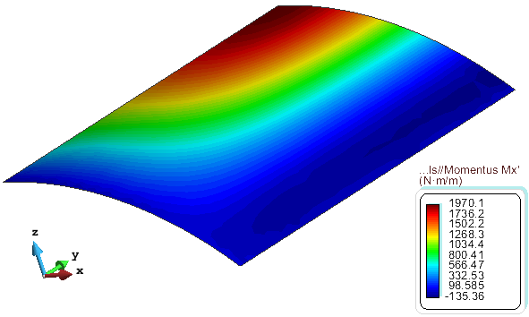
Note: See that \(M_{x'}\) momentum is contained inside plane \(X'Z'\). This criteria is different from the strength criteria in beams or in constraints, where the rotation in \(X'\) is the one that rotates around \(X'\) axe. The rotation axe criteria for shell momentum are inherited from the plate criteria. In that case, as there are only two rotations in a plate, this choosing looked appropriate. For rotations in 3D, as there are 3, it is necessary to use the other criteria.

As a example, this is the \(M_{x'}\) momentum on the shell:

Postprocess panel >> Results >> Static >> Shells >> Momentum >> Mx >> Contour fill

Shear, momentum and axial forces

The shear forces do not follow the same tensor approach because they are two forces, one for each local axis. As they can be represented in any local axes system, it is possible to see in RamSeries the shear represented in the same local axes base than the Main momentum. To do so, select:

Postprocess panel >> Results >> Static >> Shells >> Shear in main >> Qm1 – Qm2

Following the theory of elasticity, the axial force is represented in a given base \(X'Y'\) by the following tensor:

\[\begin{split}\begin{bmatrix} N_{x'} & N_{x'y'} \\ N_{x'y'} & N_{y'} \end{bmatrix}\end{split}\]

It is always possible to find another base X’’Y’’ where the tensor is represented as:

\[\begin{split}\begin{bmatrix} N_{11} & 0 \\ 0 & N_{22} \end{bmatrix}\end{split}\]

These are the eigenvalues of the matrix and the new base is made with the eigenvectors. Its values represent the maximum and the minimum axial value for that point of the shell. It is possible to see these values with:

Postprocess panel >> Results >> Static >> Shells >> Axial force >> Main stresses

Note: As the local axes system for the main axial forces change from element to element, in some cases where this change is too big the smoothing in the contour fill is not being done. For this reason, some discontinuities of the results can be appreciated.

The same ideas than for the Main axial force can be applied to the momentum. In this case, to display the main momentum use:

Postprocess panel >> Results >> Static >> Shells >> Moments >> Mi – Mii

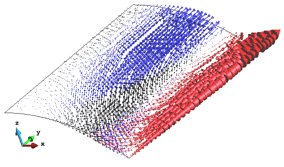
This is the reaction momentum. It is expressed as a vector showing the rotation axe and a module that means the rotation amount. Default units are \(N·m\).

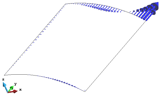
Postprocess panel >> Results >> Static >> M Reactions >> Vectors

These are the reactions that appear in the constraints. All nodes that have no constraint will have a null reaction. Default units are \(Newtons\).

Postprocess panel >> Results >> Static >> Reactions >> Vectors

If labels are displayed, four numbers appears. The first three are the reaction vector and the last is the module of this vector.