RamSeries-Tutorial 1: Analysis of a beam structure
Model case
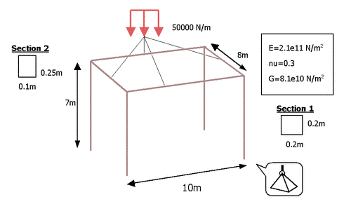
Schematic representation of the spatial frame under analysis.
Problem description
This tutorial is aimed to perform a simple structural analysis of a spatial frame subjected to the action of an homogeneous distributed load applied to the horizontal beams located at the top of the frame structure. A schematic representation of the problem under analysis is shown in the figure below. Beam’s section and material properties are also included.
The geometry can be constructed in GiD using the following useful pre-processing commands which are described in detail in the GiD User’s Manual.
Geometry >> Create >> Line >> 0,0,0 >> 10,0,0
Utilities >> Copy >> Translation
View >> Rotate >> Line >> 0,0,0 >> 10,0,0
The final model will be composed of 8 lines and all the corresponding connection points.
Problem specification
To load the RamSeries type of analysis, choose the following option in the Start Data window:
Simulation type >> Structural analysis
The same option can be alternatively activated through the data tree by using the following option:
Simulation data >> Simulation type >> Structural analysis
The kind of problem under consideration in this tutorial, requires the following basic options to be selected:
Simulation dimension: 3D
Structural analysis element types: Beams
Analysis type: Static analysis
Material constitutive model: Linear-elastic model
Geometrical constitutive model: Linear geometry
This setup can be configured from the Start Data window that can be accessed from the Data menu as follows:
Data >> Start Data
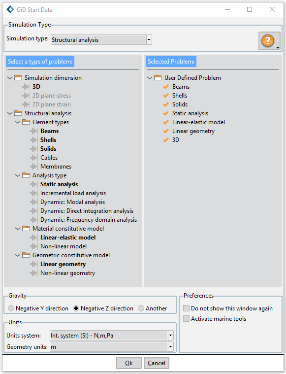
Start Data window as it appears after configuration of the type of problem required to perform structural analysis of the beams in a spatial frame structure.
Constraints
First, constraint conditions must be applied. In this case, the four inferior points of the structure have a prescription in their movements in the three global directions \(X\), \(Y\) and \(Z\). Rotations in the points are not prescribed.
Constraints >> Fixed constraints
Activation |
Values |
||
|---|---|---|---|
X constraint |
1 |
X value |
0.0 |
Y constraint |
1 |
Y value |
0.0 |
Z constraint |
1 |
Z value |
0.0 |
Rot X constr |
0 |
X value |
0.0 |
Rot Y constr |
0 |
Y value |
0.0 |
Rot Z constr |
0 |
Z value |
0.0 |
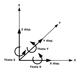
In this condition, the local axes are no related to the beam local axes defined in the properties section. The GLOBAL option means that the prescriptions assigned are related to the global axes of the problem. This is used in this case. Local axes are used to prescribe the displacement or rotation in a direction not coincident with any of the global axes. The values part of the condition is used to prescribe a fixed amount of displacement or rotation. Default units are meters for the \(X\), \(Y\) and \(Z\) displacements and radians for the prescribed rotations. In this case, the prescribed displacements and rotations are all zero. \(X\) Constraint, \(Y\) Constraint and \(Z\) Constraint mean the displacements along the axes. \(\theta_X\) constraint, \(\theta_Y\) constraints and \(\theta_Z\) constraints mean the rotations around the axes. Signs are as follows (right hand rule):
This condition must be assigned to the four points in the bottom part of the structure (minimum Z).
Material properties
Next, section and material properties must be defined. To assign the section and material properties to the beams choose:
Materials and properties >> Beams >> Rectangular section
\(W_Y = 100 \ mm\) (width of the rectangular section along the \(Y'\) direction)
\(W_Z = 250 \ mm\) (width of the rectangular section along the \(Z'\) direction)
\(E = 2.1e11 \ N/m^2\) (Young modulus)
\(G = 8.1e10 \ N/m^2\) (torsion modulus)
\(\rho = 0.0 \ N/m^3\) (the self-weight of the beam is not considered)
\(\sigma_{max} = 0.0 \ N/m^2\) (this parameter does not have influence in the calculation; it is only useful as a reference for the user when verifying stress results in postprocess).
Note: Remember that for an isotropic material: \(G=E/(2·(1+\nu))\) In this case \(\nu=0.3\)
To assign properties to the beams, it is first necessary to define local axes. To this aim, in the present case Automatic local axes ares used. Hence, following the standard criteria, \(X'\) axes (prime refers to local axes) will remain aligned along the horizontal beams longitudinal axis. On the other hand, \(Y'\) will be horizontal and perpendicular to the beam longitudinal axis, while \(Z'\) will have the same direction and sense than the global \(Z\) axis. Once the values of all rectangular section parameters have been provided, the condition must be assigned to all the horizontal beams.
When assigning the properties on the horizontal beams, the Local axes system Automatic is chosen, following the criteria given before.
The same must be made with the vertical beams. In this case the \(Y'\) axe points to the direction of the \(X\) axe, for local axes system Automatic.
The conditions that have been assigned can be viewed right-clicking on the created group:
Draw >> Draw values/groups/symbols
Load conditions
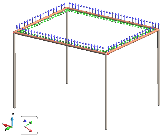
Finally the loading conditions of the problem must be specified. In the present case, all the horizontal beams have a distributed load of \(50000 \ N/m\) along the negative global \(Z-axis\). So the condition Global Beam Load will be used:
Loadcases >> Loadcase 1 >> Beams >> Pressure load
Factor |
1.0 |
Loadtype |
Global |
X pressure |
0.0 \(N/m\) |
Y pressure |
0.0 \(N/m\) |
Z pressure |
-5.0e4 \(N/m\) |
This condition shall be assigned to all the horizontal beams.
Mesh generation
For most of the geometrical models, especially if all the beams are straight, it is only necessary one beam element per line. To obtain it, generate the mesh with a big default element size. It should be chosen longer than any of the lines length. For this example 100 units can be chosen. If there are curved lines, it can be necessary to mesh several beam elements for every line. To do so, use GiD options to control the mesh size like:
Meshing >> Assign unstructured sizes >> Points Meshing >> Assign unstructured sizes >> Lines Meshing >> Assign unstructured sizes >> By chordal error
To generate the mesh use:
Meshing >> Generate >> 100
RamSeries only accepts the default 2-nodes beam elements. So quadratic option is not accepted for beams. Check the GiD manual for details.
Calculate
If the model has not been saved yet, use:
File >> Save
and give a name to the model. To begin the analysis choose:
Calculate >> Calculate
The analysis runs as a separate process. Then, it is possible to continue working with GiD or exit the program. When the analysis is finished, a window will appear notifying it. If it has not run successfully, one window showing some error info will be supplied. Correct the error and run again. It is possible to visualize, when the process is running, some information about its evolution. Press:
Calculate >> View process info
Postprocess and results analysis
The part of the program dedicated to visualize the results of the analysis is called Post-process. Once the calculation is finished, to enter in the post-process part and load automatically the results select:
Postprocess >> Start
To perform the operation correctly, it is necessary to have the model loaded inside the pre-processing part before going to post-process.
Visualization of local axes
The first important checking that must be done is to see if the local axes for every beam are equal to the ones supposed when assigning the properties. Choose:
Postprocess panel >> Results >> Automatic local axes >> Local axes mesh - beams >> Local axes
If they are different than supposed, go to the pre-processing part, change the properties accordingly and calculate again. If the drawing of the local axes appear too big or to small, the scale drawing factor may be changed by entering a different factor in:
Postprocess panel >> Preferences >> Vectors & Local axes >> Factor
Deformation results
To visualize the deformed (with displacements contour fill on it) of the structure, chose the following options:
Postprocess panel >> Meshes >> Line style >> 2nd option
Postprocess panel >> Results >> Static >> Displacements >> Contour fill
Postprocess panel >> Preferences >> Deformed >> Draw: [Yes]
Postprocess panel >> Preferences >> Deformed >> Factor: [5]
Postprocess panel >> Preferences >> Deformed >> Result: [“Static displacements”]
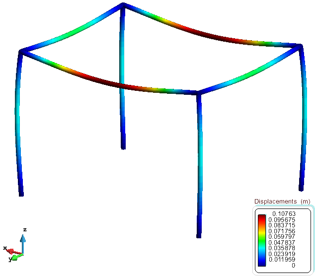
Deformed of the structure with contour fill of displacements [m]
The deformed of the structure is drawn magnified in the screen (factor 5 chosen). The magnifying factor can be automatically calculated if “Adimensional factor” is checked instead. To see the numerical values of the deformation choose at any point, node or element:
Postprocess >> Mesh information
Try also pressing mouse left button over any structure element in the screen.
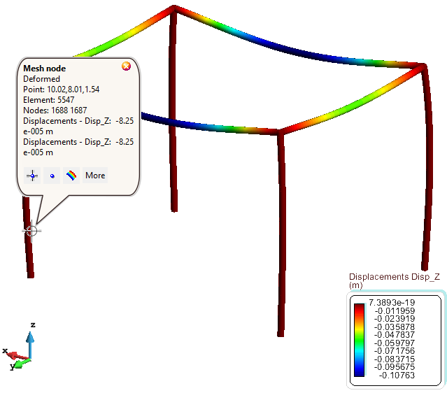
Make the appropriate zooms to visualize properly the values. The values are the maximums and lateral values of every beam and represent the vector, expressed in global coordinates, of the displacement. The default units are meters.
To switch off the labels press:
Mouse right button >> Label >> Off
In order to choose the visualization style for the diagrams, try:
Postprocess panel >> Meshes >> Line style
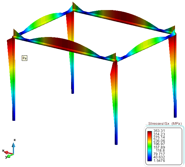
Strength results
All of the strengths are represented related to the local axes systems of every beam. The visualization is made with a diagram that will be more separated from the beam as the magnitude of the strength increases. It will be drawn in either side of the beam depending on the sign. To draw labels with the numerical value of the strength that is being visualized, press the left mouse button over the screen.
Postprocess panel >> Results >> Static >> Beams >> Max stresses >> Sx >> Line diagram
Shear, momentum and axial forces
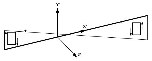
This is the shear in the X’Z’ plane. Default units are N.
Postprocess panel >> Results >> Static >> Beams >> Z’ Shear >> Line diagram
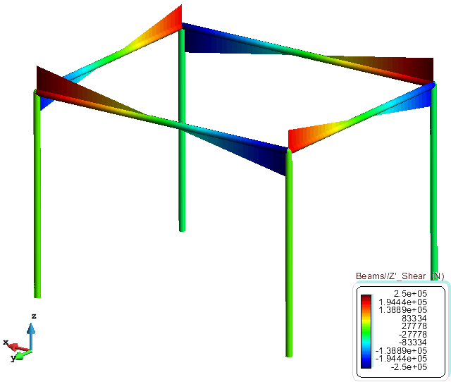
In the figure the sign criteria for the shear is shown.
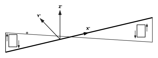
This is the shear in the X’Y’ plane. Default units are N.
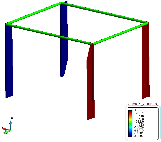
Postprocess panel >> Results >> Static >> Beams >> Y’ Shear >> Line diagram
In the figure the sign criteria for the shear is shown.
These are the reactions that appear in the constraints. All nodes that have no constraint will have a null reaction. Default units are N.
Postprocess panel >> Results >> Static >> Reactions >> Vectors
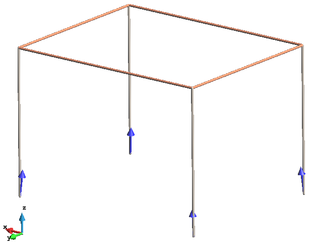
For obtaining the numerical result of all the reactions go to:
Postprocess >> Compose reactions
If labels are displayed, four numbers appears. The first three are the reaction vector and the last is the module of this vector.
This is the momentum that rotates around the Z’ axe. Default units are N·m.
Postprocess panel >> Results >> Static >> Beams >> Z’ momentum >> Line diagram
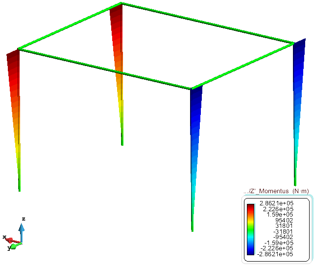
Sign criteria for Z’ momentum is:
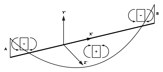
Diagram is drawn in the plane X’Y’ and in the side of the beam where the traction is. Positive values of the momentum mean that traction is in the –Y’ side (in the negative side of Y’).
This is the momentum that rotates around the Y’ axe. Default units are N·m.
Postprocess panel >> Results >> Static >> Beams >> Y’ momentum >> Line diagram
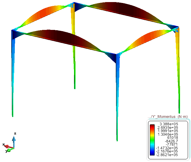
Sign criteria for Y’ momentum is:
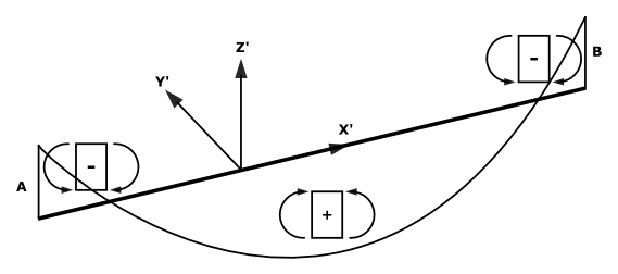
Diagram is drawn in the plane X’Z’ and in the side of the beam where the traction is. Positive values of the momentum mean that traction is in the –Z’ side (in the negative side of Z’).
This is the axial force in the beam axe. Default units are N.
Postprocess panel >> Results >> Static >> Beams >> Axial force >> Line diagram
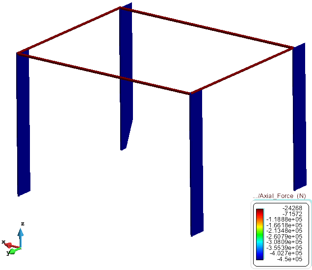
A positive value means traction in the beam. Negative means compression.