2.2.3. Overlapping domain decomposition level set (FSURF module)

This section introduces one of the algorithms implemented in Tdyn for the analysis of free surface flows. The main innovation of this method is the application of domain decomposition concept in the statement of the problem, in order to increase accuracy in the capture of free surface as well as in the resolution of governing equations in the interface between the two fluids. Free surface capturing is based on the solution of a level set equation, while Navier Stokes equations are solved using the iterative monolithic predictor-corrector algorithm presented above, where the correction step is based on the imposition of the divergence free condition in the velocity field by means of the solution of a scalar equation for the pressure.

2.2.3.1. Governing equations

The velocity and pressure fields of two incompressible and immiscible fluids moving in the domain \(\Omega \in R^d (d = 2,3)\) can be described by the incompressible Navier Stokes equations for multiphase flows, also known as non-homogeneous incompressible Navier Stokes equations:

(2.262)\[\begin{aligned} & \frac{\partial \rho }{\partial t} + \frac{\partial}{\partial x_j} \left( \rho u \right) = 0 \end{aligned}\]

(2.263)\[\begin{aligned} & \frac{\partial \rho u_i}{\partial t} + \frac{\partial}{\partial x_j} \left( \rho u_i u_j \right) + \frac{\partial p}{\partial x_i} - \frac{\partial τ_{ij}}{\partial x_j} = \rho f_i \end{aligned}\]

(2.264)\[\begin{aligned} & \frac{\partial u_i}{\partial x_j} = 0 \end{aligned}\]

Where \(1≤i\), \(j≤d\), \(\rho ` is the fluid density field, :math:`u_i\) is the ith component of the velocity field \(u\) in the global reference system \(x_i\), \(p\) is the pressure field and \(\tau\) is the viscous stress tensor defined by

(2.265)\[\begin{aligned} & τ_{ij} = \mu \left( \partial_i u_j + \partial_j u_i \right) \end{aligned}\]

where \(\mu\) is the dynamic viscosity.

Let \(\Omega_1 = {x \in \Omega | x \in \text{ Fluid1}}\) be the part of the domain \(\Omega\) occupied by the fluid number \(1\) and let \(\Omega_2 = {x \in \Omega | x \in \text{ Fluid2}}\) be the part of the domain \(\Omega\) occupied by fluid number \(2\). Therefore \(\Omega_1\), \(\Omega_2\) are two disjoint subdomains of \(\Omega\). Therefore (see Figure 4)

(2.266)\[\begin{aligned} & \Omega = int \left( \overline{ \Omega_1 ∩ \Omega_2 } \right) \end{aligned}\]

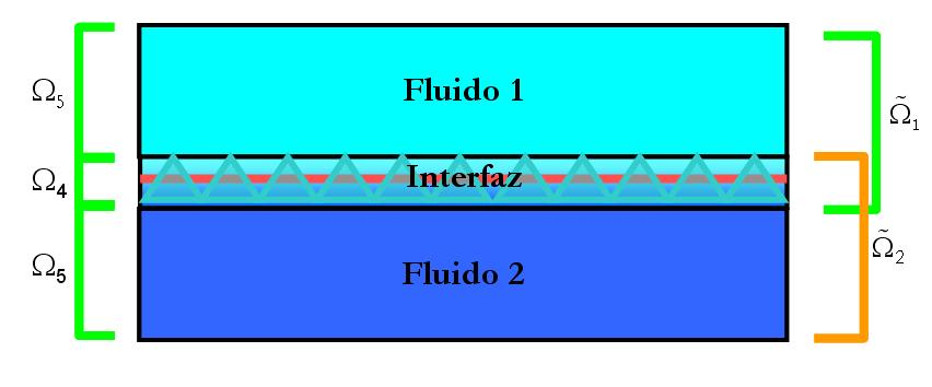
Fig. 2.16 Domain decomposition

where ‘int’ denotes the topological interior and the over bar indicates the topological adherence of a given set, for more details see [García_2008]. The system in Eq. (3-1) must be completed with the necessary initial and boundary conditions, as shown below. It is usual in the literature to consider that the first equation in Eq. (3-1) is equivalent to impose a divergence free velocity field, since the density is taken as a constant. However, in the case of multiphase incompressible flows, density cannot be consider constant in \(\Omega \times (0,T)\). Actually, it is possible to define \(\rho\), \(\mu\) fields as follows:

(2.267)\[\begin{split}\begin{aligned} & \rho , \mu = \left\{ \begin{matrix} \rho _1, \mu_1 & x \in \Omega_1 \\ \rho _2, \mu_2 & x \in \Omega_2 \\ \end{matrix} \right\} \end{aligned}\end{split}\]

Let \(\Psi ∶ \Omega \times (0,T)→R\) be a function (named Level Set function) defined as follows:

(2.268)\[\begin{split}\begin{aligned} & \Psi (x,t) = \left\{ \begin{matrix} d(x,t) & x \in \Omega_1 \\ 0 & x \in \Gamma \\ -d(x,t) & x \in \Omega_2 \\ \end{matrix} \right\} \end{aligned}\end{split}\]

Where \(d(x,t)\) is the distance to the interface between the two fluids, denoted by \(\Gamma\), of the point \(x\) in the time instant \(t\). From the above definition it is trivially obtained that:

(2.269)\[\begin{aligned} & \Gamma = \left\{ x \in \Omega | \Psi(x,\cdot ) = 0 \right\} \end{aligned}\]

Since the level set \(0\) identifies the free surface between the two fluids, the following relations can be obtained:

(2.270)\[\begin{aligned} & n(x,t) = \nabla \Psi|_{(x,t)} & ; \kappa(x,t) = \nabla \cdot (n(x,t)) \end{aligned}\]

Where \(n\) is the normal vector to the interface \(\Gamma\), oriented from fluid 1 to fluid 2 and \(\kappa\) is the curvature of the free surface. In order to obtain the above relations it has been assumed that function \(\Psi\) fulfils:

(2.271)\[\begin{aligned} & |\nabla \Psi| = 1 & ∀ (x,t) \in \Omega \times (0,T) \end{aligned}\]

Therefore, it is possible to redefine density and viscosity as follows:

(2.272)\[\begin{split}\begin{aligned} & \rho , \mu = \left\{ \begin{matrix} \rho _1, \mu_1 & \Psi > 0 \\ \rho _2, \mu_2 & \Psi < 0 \\ \end{matrix} \right\} \end{aligned}\end{split}\]

Let us write the density fields in terms of the level set function \(\Psi\) as

(2.273)\[\begin{aligned} & \rho (x,t) = \rho \left( \Psi(x,t) \right) & ∀ (x,t) \in \Omega \times (0,T) \end{aligned}\]

Then, density derivatives can be written as

(2.274)\[\begin{split}\begin{aligned} & \frac{\partial \rho }{\partial t} = \frac{\partial \rho }{\partial \Psi} \frac{\partial \Psi}{\partial t} \\ & \frac{\partial \rho }{\partial x_i} = \frac{\partial \rho }{\partial \Psi} \frac{\partial \Psi}{\partial x_i} \end{aligned}\end{split}\]

Inserting the above relation into the first line of Eq. (3-1) gives

(2.275)\[\begin{split}\begin{aligned} & \frac{\partial \rho }{\partial t} + \frac{\partial}{\partial x_i} \left( \rho u_i \right) = \frac{\partial \rho }{\partial t} + u_i \frac{\partial \rho }{\partial x_i} = \frac{\partial \rho }{\partial \Psi} \frac{\partial \Psi}{\partial t} + \frac{\partial \rho }{\partial \Psi} u_i \frac{\partial \Psi}{\partial x_i} = \\ & = \frac{\partial \rho }{\partial \Psi} \left[ \frac{\partial \Psi}{\partial t} + u_i \frac{\partial \Psi}{\partial x_i} \right] = 0 \end{aligned}\end{split}\]

which gives as a result that the multiphase Navier Stokes problem is equivalent to solve the following system of equations:

(2.276)\[\begin{aligned} & \frac{\partial \rho u_i}{\partial t} + \frac{\partial}{\partial x_j} \left( \rho u_i u_j \right) + \frac{\partial p}{\partial x_i} - \frac{\partial τ_{ij}}{(\partial x_j} = \rho f_i \end{aligned}\]

(2.277)\[\begin{aligned} & \frac{\partial u_i}{\partial x_i} = 0 \end{aligned}\]

coupled with the equation

(2.278)\[\begin{aligned} & {\partial \Psi}{\partial t} + u_i \frac{\partial \Psi}{\partial x_i} = 0 \end{aligned}\]

Eq. (3-14) defines the transport of the level set function due to the velocity field obtained by solving Eq. (3-13). As a conclusion, the free surface capturing problem can be described by the above equations. In this formulation, the interface between the two fluids is defined by the level \(0.5\) of \(\Psi\).

Denoting prescribed values by an over-bar, the boundary conditions to be considered for the above presented problem are:

(2.279)\[\begin{aligned} & u = \overline{u} & \text{in } \Gamma_u \end{aligned}\]

(2.280)\[\begin{aligned} & p = \overline{p}, & n_j τ_{ij} = \overline{t}_i & \text{ in } \Gamma_p \end{aligned}\]

(2.281)\[\begin{split}\begin{aligned} & u_j n_j= \overline{u}_n , & \left\{ \begin{matrix} n_j \tau_{ij} g_i = \overline{t}_1 \\ n_j \tau_{ij} s_i = \overline{t}_2 \\ \end{matrix} \right\} & \text{in } \Gamma_{\tau} \end{aligned}\end{split}\]

Where the boundary \(\partial \Omega\) of the domain \(\Omega\) has been split in three disjoint sets: \(\Gamma _u\), \(\Gamma _p\) where the Dirichlet and Neumann boundary conditions are imposed and \(\Gamma _τ\) where the Robin conditions for the velocity are set. In the above, vectors \(g\), \(s\) span the space tangent to \(\Gamma _τ\). In a similar way, the boundary conditions for Eq. (3-14) are defined

(2.282)\[\begin{aligned} & \Psi = \overline{\Psi} & \text{in } \Gamma_u \end{aligned}\]

Finally, the initial conditions of the problem are

(2.283)\[\begin{aligned} & u = u_0 & \text{in } \Omega , & \Psi = \Psi_0 & \text{in } \Omega \end{aligned}\]

Where \(\Gamma_0 = \left\{ x \in \Omega | \Psi_0 (x) = 0 \right\}\) defines the initial position of the free surface between the two fluids.

2.2.3.2. How to calculate a signed distance to the interface

Based on flow properties as density or viscosity, we can calculate an initial guess for \(\Psi\) as follows:

(2.284)\[\begin{split}\begin{aligned} & \Psi(x,t) = \left\{ \begin{matrix} 1 & \text{if } \rho (x,t) = \rho _1 \\ 0 & \text{if } x \in \Gamma(t) \\ -1 & \text{if } \rho (x,t) = \rho _2 \\ \end{matrix} \right\} \end{aligned}\end{split}\]

Clearly, the level set function obtained from Eq. (3-18) is not a signed distance to \(\Gamma\). We need to reinitiate \(\Psi\) in order to guarantee that \(\Psi\) fulfils the definition. We use a technique based on the following property to reinitiate the level set function as a signed distance to \(\Gamma\). If \(\Psi\) is a signed distance function to \(\Gamma\) then,

(2.285)\[\begin{aligned} & ‖ \nabla \Psi ‖ = 1 & ∀ (x,t) \in \Omega \times (0,T] \end{aligned}\]

where \(‖\cdot ‖\) denotes the Euclidian norm in \(R^d\).

We use Eq. (3-19) to recalculate \(\Psi\). In case that Eq. (3-19) is not satisfied, then

(2.286)\[\begin{aligned} & 1 - ‖ \nabla \Psi ‖ = r \end{aligned}\]

The residual \(r\) in Eq. (3-20) can be understood as the time derivate of \(\Psi\) with respect to a pseudo-time \(\tau\), i.e.

(2.287)\[\begin{aligned} & r ∶= \partial _{\tau} \Psi \end{aligned}\]

Then, the stationary solutions of Eq. (3-21) (i.e. when \(\partial _{\tau} \Psi = 0\)) satisfy Eq. (3-19). In summary, for a given time \(t \in [0,T]\), we calculate \(\Psi\) as the stationary solution of the following hyperbolic problem.

(2.288)\[\begin{split}\begin{aligned} & \partial_{\tau} \Psi + ‖ \nabla \Psi ‖ = 1 & \text{in } \Omega \\ & \Psi (\tau = 0) = \Psi(\cdot,t) \\ & \Psi (x,\tau) = 0 & ∀ x \text{ in } \Gamma (t) \end{aligned}\end{split}\]

The problem stated in Eq. (3-22) can be rewritten in a more convenient manner as

(2.289)\[\begin{aligned} & \partial_{\tau} \Psi + \left( \boldsymbol{w} \cdot \nabla \right) \Psi = sign \left( \Psi \right); & \boldsymbol{w} = sign \left( \Psi \right) \frac{\nabla \Psi}{‖ \nabla \Psi‖} \end{aligned}\]

Since the level set values identify the free surface between the two fluids, the following relations can be obtained:

(2.290)\[\begin{aligned} & \boldsymbol{n}(\boldsymbol{x},t) = \nabla \Psi |_{x,t} & ; & \kappa(\boldsymbol{x},t) = \nabla \cdot \left( \boldsymbol{n}(\boldsymbol{x},t) \right) \end{aligned}\]

where \(\boldsymbol{n}\) is the normal vector to the interface \(\Gamma\), oriented from fluid 2 to fluid 1 and \(\kappa\) is the local curvature of the interface.

From equation Eq. (3-23) it can be easily shown that the reinitialization process begins from the interface and it propagates to the whole domain. This property is attractive from the computational point of view, since we are only interested in accurate values of \(\Psi\) in the region close to the interface. Then we only need to reach the steady state solution of Eq. (3-23) in a narrow band close to the interface as proposed in [García_2003]. The reinitialization algorithm used in this work has been optimized using the concept of nodal levels described next.

Given a level set distribution \(\Psi\), for every time step \(t\) one can assign a level \(l_i\) to the node \(x_i\) based on the following rules:

• A nodal point \(i\) of coordinates \(x_i\) belongs to the level \(l_i=1\), if \(\Psi(x_i,t)≥0\), and it is connected to at least one node \(j\) with \(\Psi(x_j,t)<0\)

• A nodal point \(i\) of coordinates \(x_i\) belongs to the level \(l_i= -1\), if \(\Psi(x_i,t)<0\), and it is connected to at least one node \(j\) with \(\Psi(x_j,t)≥0\)

• A nodal point \(i\) of coordinates \(x_i\) belongs to the level \(l_i>1\), if \(\Psi(x_i,t)>0\), and it is connected to at least one node of level \(l_(i-1)\)

• A nodal point \(i\) of coordinates \(x_i\) belongs to the level \(l_i<-1\), if \(\Psi(x_i,t)<0\), and it is connected to at least one node of level \(l_(i+1)\)

Once the levels have been assigned to the mesh points, the reinitialization is performed in a narrow band of \(n\) levels around the interface. Eq. (3-23) is solved using a forward Euler scheme until the steady state in the \(n\) levels is achieved. \(k\) iterations with \(k > n\) are performed in such a way that for every iteration \(i = 1,…,k\). The iterations are carried out only for those nodes \(j\) of the mesh with \(|l_j| ≤ i\). Due to the evolution of the interface defined by Eq. (3-14), the level set function does not fulfil Eq. (3-19) after some time. It is therefore recommended to apply the reinitialization scheme described above at every time step.

2.2.3.3. Interfacial boundary conditions

At a moving interface the jump condition applies. For immiscible fluids we can write:

(2.291)\[\begin{split}\begin{aligned} & \left[ \boldsymbol{n} \cdot \left( \boldsymbol{\sigma} \cdot \boldsymbol{n} \right) \right] = \gamma \kappa & \text{in } \Gamma \\ & \left[ \boldsymbol{s} \cdot \left( \boldsymbol{\sigma} \cdot \boldsymbol{n} \right) \right] = 0 & \text{in } \Gamma \\ \end{aligned}\end{split}\]

where \(\gamma\) is the coefficient of surface tension (a constant of the problem), \(\boldsymbol{s}\) is any unit vector tangent to the interface and \([\cdot]\) defines the jump across the interface.

(2.292)\[\begin{aligned} & \left[ A \right] = A_1 - A_2 \end{aligned}\]

Taking into account that \(\boldsymbol{\sigma}_i = -p I + \mu_i \left( \nabla u + \nabla u^T \right) , i = 1, 2\) and using \(\cdot n=0\) , the second equation in Eq. 67 yields

(2.293)\[\begin{aligned} & \boldsymbol{s} \cdot \left[ \left( \mu_1 - \mu_2 \right) \left( \nabla u + \nabla u^T \right) \cdot \boldsymbol{n} \right] = 0 \end{aligned}\]

From Eq. (3-27) we can conclude that \(\left( \mu_1 - \mu_2 \right) \left( \nabla u + \nabla u^T \right) \cdot n \in 〈s〉^⊥\), where \(〈v〉^⊥\), denotes the orthogonal subspace to \(v\). Then it is clear that

(2.294)\[\begin{aligned} & \left( \mu_1 - \mu_2 \right) \left( \nabla \boldsymbol{u} + \nabla \boldsymbol{u}^T \right)\cdot \boldsymbol{n} = \lambda \boldsymbol{n} & , & \lambda \in Spec(\tau_1 - \tau_2) \end{aligned}\]

Integrating over any closed surface \(\partial M\) containing \(\Gamma\) in both sides of Eq. (3-28) yields

(2.295)\[\begin{aligned} & \int_{\partial M} ( \mu_1 - \mu_2 ) \boldsymbol{n} \cdot ( \nabla u + \nabla u^T ) = \int_{\partial M} \lambda \boldsymbol{n} \end{aligned}\]

Applying the Gauss theorem to the right hand side of Eq. (3-29) we can deduce that \(\lambda = 0\) or equivalently

(2.296)\[\begin{aligned} & \boldsymbol{n} \cdot ( \nabla u + \nabla u^T ) & \text{in } \Gamma \end{aligned}\]

Introducing Eq. (3-30) into the first condition in Eq. (3-25) the following equivalent condition is obtained:

(2.297)\[\begin{aligned} & p_1 \boldsymbol{n} = p_2 \boldsymbol{n} + \gamma \kappa \boldsymbol{n} \end{aligned}\]

This form of the jump condition is very useful in the development of the method presented in the following sections. In the classical level set formulation for multiphase flow problems [Zienkiewicz_1995] the jump condition Eq. (3-25) can be introduced into the momentum equation by adding an additional source term, i.e.

(2.298)\[\begin{split}\begin{aligned} & \partial_t \left( \rho \boldsymbol{u} \right) + \nabla \left( \rho \boldsymbol{u} ⨂ \boldsymbol{u} \right) - \nabla \boldsymbol{\sigma} = \rho \tilde{f} \\ & \tilde{f} = f + \gamma \kappa \boldsymbol{n} \delta(\Gamma) \end{aligned}\end{split}\]

Where \(\delta(\Gamma)\) is a Dirac’s delta function on \(\Gamma\). Since the properties of the fluids change discontinuously across the interface, the direct solution of Eq. (3-32) has important numerical drawbacks: inaccurate resolution of the pressure at the interface, fluid mass losses, inaccurate interface location, etc. A common approach to overcome these difficulties is to smooth the discontinuous transition of the flow properties and the Dirac’s delta functions across the interface using of a smoothed Heaviside function. This function is usually expressed as:

(2.299)\[\begin{split}\begin{aligned} & H_{\epsilon} \left( \Psi \right) = \left\{ \begin{matrix} 0 & \Psi < - \epsilon \\ \frac{1}{2} \left[ 1 + \frac{\Psi}{\epsilon} + \frac{1}{\pi} sin \left( \frac{\pi \Psi}{\epsilon} \right) \right] & |\Psi| ≤ \epsilon \\ 1 & \Psi > \epsilon \\ \end{matrix} \right\} \end{aligned}\end{split}\]

where \(2\epsilon\) is the thickness of the transition area. Then a property \(\eta\) is approximated as

(2.300)\[\begin{aligned} & \eta(ϕ) = \eta_1 + (\eta_1 - \eta_2 ) H_\epsilon (ϕ) \end{aligned}\]

and a Dirac’s delta function as

(2.301)\[\begin{aligned} & \delta(\Gamma) = d_{\Psi} H_\epsilon \end{aligned}\]

This approach also presents several deficiencies: the accuracy of the results depends on the ad hoc thickness of the transition area \(2\epsilon\), the jump condition is not properly captured, the interface propagation velocity is not correctly calculated, etc.

Other schemes, such as the Ghost Cell method or lagrangian methods as the Particle FEM Method, attempt to overcome the problem of properties smoothing at the interface region. However, these methods have several drawbacks, such us limitations of conservative and convergence properties in some cases or an increase of the computational effort. As a conclusion, a method able to deal with a discontinuous transition of properties across the interface, the jump interface condition and computationally affordable for large models is required.

The overlapping domain decomposition method described in the following sections has been developed to overcome these difficulties.

2.2.3.4. Stabilized FIC-FEM formulation

The stabilized FIC form of the governing differential equations Eq. (3-13) and Eq. (3-14) is written as

(2.302)\[\begin{split}\begin{aligned} & r_m - \underline{ \frac{1}{2} \left( h_m \cdot \nabla \right) r_m } = 0 \\ & r_d - \underline{ \frac{1}{2} \left( h_d \cdot \nabla \right) r_d } = 0 \\ & r_{\Psi} - \underline{ \frac{1}{2} \left( h_{\Psi} \cdot \nabla \right) }= 0 \\ \end{aligned}\end{split}\]

The boundary conditions for the stabilized FIC problem are written as

(2.303)\[\begin{aligned} & \boldsymbol{u} = \overline{\boldsymbol{u}} & \text{in } \Gamma_D \end{aligned}\]

(2.304)\[\begin{aligned} & \boldsymbol{n} \cdot \boldsymbol{\sigma} - \underline{ \frac{1}{2}\boldsymbol{n} \cdot \boldsymbol{h}_m \cdot \boldsymbol{r}_m } = \overline{t} & \text{in } \Gamma_N \end{aligned}\]

(2.305)\[\begin{aligned} & \boldsymbol{n} \cdot \boldsymbol{u} = \overline{u}_n, & \boldsymbol{n} \cdot \boldsymbol{\sigma} \cdot \boldsymbol{g} \underline{ - \frac{1}{2} \boldsymbol{n} \cdot \boldsymbol{h}_m \cdot \boldsymbol{r}_m \cdot \boldsymbol{g} } = \overline{\boldsymbol{t}}_1 & \text{in } \Gamma_M \end{aligned}\]

(2.306)\[\begin{aligned} & \boldsymbol{n} \cdot \boldsymbol{\sigma} \cdot \boldsymbol{s} \underline{ - \frac{1}{2} \boldsymbol{n} \cdot \boldsymbol{h}_m \cdot \boldsymbol{r}_m \cdot \boldsymbol{s} } = \overline{\boldsymbol{t}}_2 \end{aligned}\]

(2.307)\[\begin{aligned} & \Psi = \overline{\Psi} & \text{in } \Gamma_{inlet} \end{aligned}\]

The underlined terms in Eq. (3-36) and Eq. (3-37) introduce the necessary stabilization for the numerical solution of the Navier Stokes problem [García_1999], [Kleinstreuer_1997], [García_1998].

Note that terms \(\boldsymbol{r}_m\), \(\boldsymbol{r}_d\) and \(\boldsymbol{r}_{\Psi}\) denote the residuals of Eq. (3-13) and Eq. (3-14), i.e.

(2.308)\[\begin{aligned} & \boldsymbol{r}_m ∶= \partial _t (\rho \boldsymbol{u}) + \nabla \cdot (\rho \boldsymbol{u} ⨂ \boldsymbol{u}) + \nabla p - \nabla \cdot \boldsymbol{\sigma} - \rho \boldsymbol{f} \end{aligned}\]

(2.309)\[\begin{aligned} & \boldsymbol{r}_d = \nabla \cdot \boldsymbol{u} \end{aligned}\]

(2.310)\[\begin{aligned} & \boldsymbol{r}_{\Psi} ∶= \partial_t \Psi + (\boldsymbol{u} \cdot \nabla)\Psi \end{aligned}\]

The characteristic lengths vectors \(\boldsymbol{h}_m\), \(\boldsymbol{h}_d\) and \(\boldsymbol{h}_{\Psi}\) contain the dimensions of the finite space domain where the balance laws of mechanics are enforced. At the discrete level these dimensions are of the order of the element or grid dimension used for the computation. Details on obtaining the FIC stabilized equations and the recommendation for computing the characteristic length vectors can be found in [Oñate_1999], [García_1998] and [Oñate_2000].

2.2.3.5. Overlapping domain decomposition method

To overcome the drawbacks related to the discontinuity of fluid properties across the interface and to impose the interfacial boundary condition we split the domain \(\Omega\) into two overlapping subdomains. Based on this subdivision of the domain, we apply a Dirichlet-Neumann overlapping domain decomposition technique with appropriate boundary conditions in order to satisfy the interfacial condition. Let \(K = \cup_{e=1}^{\# K} \left( N^e, K^e, \Theta^e \right)\) be a finite element partition of the domain \(\Omega\), where \(N^e\) are element nodes, \(K^e\) is the element spatial domain, \(\Theta^e\) are element shape functions and \(K\) is the total number of elements in the partition.

We assume that \(K\) satisfies the following approximation property:

(2.311)\[\begin{aligned} & dist \left( \partial \Omega, \partial \left(\cup_{e=1}^{\# K} K^e \right) \right) ≤ max_{1 ≤ e≤ \# K}⁡ \left\{ diam(K^e) \right\} \end{aligned}\]

for a fixed instant \(t\), \(t \in (0,T]\). Let us consider a domain decomposition of domain \(\Omega\) into three disjoint subdomains \(\Omega_3 (t)\), \(\Omega_4 (t)\) and \(\Omega_5 (t)\) in such a way that \(\Omega_3 (t) = \cup_e K_3^e\), \(\Omega_5 (t) = \cup_e K_5^e\), where \(K_e^3\) are the elements of the finite element partition \(K\), such as \(\forall \boldsymbol{x} \in K_3^e | \Psi (x,t) > 0\) and \(K_e^5\) are the elements of the finite element partition such as \(\forall \boldsymbol{x} \in K_5^e | \Psi (x,t) < 0\). The geometrical domain decomposition is completed with

(2.312)\[\begin{aligned} & \Omega_4 (t) = \Omega / \left( \Omega_3 (t) \cup \Omega_5 (t) \right) \end{aligned}\]

From this partition we define the two overlapping domains:

(2.313)\[\begin{aligned} & \overline{\Omega}_1 (t) := int \left( \overline{ \Omega_3 (t) \cup \Omega_4 (t) } \right), & \overline{\Omega}_2 (t) := int \left( \overline{ \Omega_4 (t) \cup \Omega_5 (t) } \right) \end{aligned}\]

Some comments about the \(\tilde{\Omega}_1 - \tilde{\Omega}_2\) partition are given next. In order to simplify the notation we will omit the time dependency of domains in the rest of the section.

Let \(\partial \tilde{\Omega}_i , i = 1, 2\) be the boundary of \(\tilde{\Omega}_i\), then:

(2.314)\[\begin{aligned} & \partial{\tilde{\Omega}_i} \cap \partial \Omega = \underbrace{\partial \tilde{\Omega}_i \cap \Gamma_D}_{\Gamma_{iD}} \cup \underbrace{\partial \tilde{\Omega}_i \cap \Gamma_N}_{\Gamma_{iN}} \cup \underbrace{\partial \tilde{\Omega}_i \cap \Gamma_M}_{\Gamma_{iM}} \end{aligned}\]

It has to be noted that contains an additional term that is not included into . This term comes from the presence of an interface inside . Since we are using a capturing technique, the position of the interface will not lay on mesh nodes, as usually happens in a tracking technique. Therefore some elements can be intersected by the interface. Then \(\tilde{\Gamma}_i\) is defined as follows:

(2.315)\[\begin{aligned} & \tilde{\Gamma}_i = \partial \Omega_4 \cap \tilde{\Omega}_{i+(-1)^{i-1}} \end{aligned}\]

Note that \(\tilde{\Gamma}_i\) is not coincident with \(\Gamma\), but the following condition is satisfied:

(2.316)\[\begin{aligned} & dist \left( \Gamma, \tilde{\Gamma}_i \right) ≤ max⁡ \left\{ diam(K^e)|K^e \in \Omega_4 \right\} \end{aligned}\]

Summarizing, we have

(2.317)\[\begin{aligned} & \partial \tilde{\Omega}_i = \Gamma_{iD} \cup \Gamma_{iN} \cup \Gamma_{iM} \cup \tilde{\Gamma}_i \end{aligned}\]

Figure 5 is a sketch of the domain partition described above.

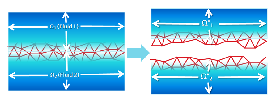
Fig. 2.17 Geometrical domain decomposition

We have two restrictions for the definition of the boundary condition on \(\tilde{\Gamma}_i\) : fluid velocities must be compatible at the interface and the jump boundary condition Eq. (3-25) must be satisfied on \(\Gamma\) . The domain decomposition technique chosen is of Dirichlet-Neumann type and it allows us to fulfil both restrictions.

Let us introduce a standard notation. We denote by \(x_i\) a variable related to \(\tilde{\Omega}_i\). For example \(\boldsymbol{u}_1\) is the velocity field solution of the problem in Eq. (3-37), where the domain \(\Omega\) has been replaced by \(\tilde{\Omega}_1\). We apply the Dirichlet conditions on \(\tilde{\Gamma}_1\) and the Neumann conditions on \(\tilde{\Gamma}_2\). For the boundary \(\tilde{\Gamma}_1\), we make use of the compatibility of velocities at the interface:

(2.318)\[\begin{aligned} & \boldsymbol{u}_1 = \boldsymbol{u}_2 & \text{in } \tilde{\Gamma}_1 \end{aligned}\]

For the boundary \(\tilde{\Gamma}_2\) we make use of the jump boundary condition. We are looking for a traction vector \(\tilde{\boldsymbol{t}}\) such that:

(2.319)\[\begin{aligned} & \boldsymbol{n}_2 \cdot \boldsymbol{\sigma}_2 = \tilde{\boldsymbol{t}} & \text{in } \tilde{\Gamma}_2 \end{aligned}\]

and \(\tilde{\boldsymbol{t}}\) must guarantee that the jump boundary condition Eq. (3-25) holds, that is to say:

(2.320)\[\begin{aligned} & p_1 \boldsymbol{n} = p_2 \boldsymbol{n} + \gamma \kappa \boldsymbol{n} & \text{in } \Gamma \end{aligned}\]

Let us write the variational problem considering the domain decomposition above described.

Domain 1:

(2.321)\[\begin{split}\begin{aligned} & \left( \rho _1 \partial_t \boldsymbol{u}_1, \boldsymbol{v} \right)_{\tilde{\Omega}_1} + \left< \rho _1 \left( \boldsymbol{u}_1 \cdot \nabla \right) \boldsymbol{u}_1, \boldsymbol{v} \right>_{\tilde{\Omega}_1} + \left( \boldsymbol{\sigma}_1, \nabla \boldsymbol{v} \right)_{\tilde{\Omega}_1} + \frac{1}{2} \left( r_{1m}, \left( h_{1m} \cdot \nabla \right) \boldsymbol{v}\right)_{\tilde{\Omega}_1} + \\ & + \left( \tilde{\boldsymbol{t}}, \boldsymbol{v} \right)_{\Gamma_{1N}} + \left( \tilde{\boldsymbol{t}_1} \boldsymbol{g} + \tilde{\boldsymbol{t}}_2 \boldsymbol{s}, \boldsymbol{v} \right)_{\Gamma_{1M}} = \left< \rho _1 \boldsymbol{f}, \boldsymbol{v} \right>_{\tilde{\Omega}_1} \end{aligned}\end{split}\]

(2.322)\[\begin{aligned} & \left( q, \nabla \cdot \boldsymbol{u}_1 \right)_{\tilde{\Omega}_1} + \frac{1}{2} \left( r_{1d}, \left(\boldsymbol{h}_{1d} \cdot \nabla \right) q \right)_{\tilde{\Omega}_1} = 0 \end{aligned}\]

(2.323)\[\begin{aligned} & \boldsymbol{u}_1 = \boldsymbol{u}_2 & \text{in } \tilde{\Gamma}_1 \end{aligned}\]

Domain 2:

(2.324)\[\begin{split}\begin{aligned} & \left( \rho _2 \partial_t \boldsymbol{u}_2, \boldsymbol{v} \right)_{\tilde{\Omega}_2} + \left< \rho _2 \left( \boldsymbol{u}_2 \cdot \nabla \right) \boldsymbol{u}_2, \boldsymbol{v} \right>_{\tilde{\Omega}_2} + \left( \boldsymbol{\sigma}_2, \nabla \boldsymbol{v} \right)_{\tilde{\Omega}_2} + \frac{1}{2} \left( r_{2m}, \left( h_{2m} \cdot \nabla \right) \boldsymbol{v}\right)_{\tilde{\Omega}_2} + \\ & + \left( \tilde{\boldsymbol{t}}, \boldsymbol{v} \right)_{\Gamma_{2N}} + \left( \tilde{\boldsymbol{t}_1} \boldsymbol{g} + \tilde{\boldsymbol{t}}_2 \boldsymbol{s}, \boldsymbol{v} \right)_{\Gamma_{2M}} = \left< \rho _2 \boldsymbol{f}, \boldsymbol{v} \right>_{\tilde{\Omega}_2} \end{aligned}\end{split}\]

(2.325)\[\begin{aligned} & \left( q, \nabla \cdot \boldsymbol{u}_2 \right)_{\tilde{\Omega}_2} + \frac{1}{2} \left( r_{2d}, \left(\boldsymbol{h}_{2d} \cdot \nabla \right) q \right)_{\tilde{\Omega}_2} = 0 \end{aligned}\]

An iterative strategy between the two domains is used to reach a converged global solution in the whole domain \(\Omega\). It is expected that this global solution will satisfy both restrictions presented above. For this reason we define the following stop criteria:

(2.326)\[\begin{split}\begin{aligned} & ‖ u_1 - u_2 ‖ ≤ tol_u & \text{in } \Omega \\ & | \boldsymbol{n} \cdot \left( \boldsymbol{\sigma}_1 - \boldsymbol{\sigma}_2 \right) \cdot \boldsymbol{n} - \gamma \kappa | ≤ tol_{\sigma} & \text{in } \Gamma \end{aligned}\end{split}\]

The global velocity solution obtained from Eq. (3-49) is used as the convective velocity for the transport of the level set function, i.e.

(2.327)\[\begin{aligned} & \left( \partial_t \Psi, ζ \right)_{\Omega} + \left< \left( \boldsymbol{u} \cdot \nabla \right) \Psi, ζ \right>_{\Omega} + \frac{1}{2} \left( r_{\Psi}, \left( h_{\Psi} \cdot \nabla \right) ζ \right)_{\Omega} = 0 \end{aligned}\]

Unfortunately there is not theoretical result that can ensure the convergence of this method. However our experience in applying this method to a wide range of problems involving moving interfaces has showed that the method is stable and robust.

An expected property of the method is its dependency with the mesh size around the interface. This issue is directly related with how good is approximated by , as it has been point out in property Eq. (3-44). A fine mesh close to the interface reduces significantly the amount of iterations needed to reach a converged global solution, as well as the accuracy of the velocities and the pressure at the interface.

This methodology can be viewed as a combination of domain decomposition and level set techniques. This justifies the name given to the new method: ODDLS (by Overlapping Domain Decomposition Level Set).

2.2.3.6. Discretization by the finite element method (FEM)

In this section we present the final discrete system of equations associated to the problem defined by Eq. (3-48) and Eq. (3-49) using the FEM method. Let us consider a uniform partition of the time interval of analysis \([0, T]\), with time step size \(\delta t\). We will denote by a superscript the time step at which the algorithmic solution is computed. We assume \(\boldsymbol{u}_1^n\), \(p_1^n\), \(\boldsymbol{u}_2^n\) and \(p_2^n\) are known. If \(\theta \in [0,1]\), the trapezoidal rule applied to Eq. (3-48) and Eq. (3-49) consists in finding \(\boldsymbol{u}_1^{n+1}\), \(p_1^{n+1}\), \(\boldsymbol{u}_2^{n+1}\) and \(p_2^{n+1}\) as the solution of the problem

(2.328)\[\begin{split}\begin{aligned} & \left( \rho _i^n \Delta _t \boldsymbol{u}_i^n, \boldsymbol{v} \right)_{\tilde{\Omega}_i} + \left< \rho _i^n \left( \boldsymbol{u}_i^{n+\theta} \cdot \nabla \right) \boldsymbol{u}_i^{n+\theta}, \boldsymbol{v} \right>_{\tilde{\Omega}_i} + \left( \sigma_i^{n+\theta}, \nabla \boldsymbol{v} \right)_{\tilde{\Omega}_i} + \\ & + \frac{1}{2} \left( r_{im}^{n+\theta}, \left( h_{im}^{n+\theta} \cdot \nabla \right) \boldsymbol{v} \right)_{\tilde{\Omega}_i} + \left(\tilde{\boldsymbol{t}}, \boldsymbol{v} \right)_{\Gamma_{iN}} + \left( \tilde{\boldsymbol{t}}_1 \boldsymbol{g} + \tilde{\boldsymbol{t}}_2 \boldsymbol{s}, \boldsymbol{v} \right)_{\Gamma_{iM}} + \left( i - 1 \right) \left( \tilde{\boldsymbol{t}}, \boldsymbol{v} \right)_{\tilde{\Gamma}_i} = \\ & = \left< \rho _i^n \boldsymbol{f},\boldsymbol{v} \right>_{\tilde{\Omega}_i} \end{aligned}\end{split}\]

(2.329)\[\begin{aligned} & \left( q, \nabla \cdot \boldsymbol{u}_i^{n+\theta} \right)_{\tilde{\Omega}_i} + \frac{1}{2} \left( r_{id}^{n+\theta}, \left(h_{im}^{n+\theta} \cdot \nabla \right) q \right)_{\tilde{\Omega}_i} = 0 & i = 1, 2 \end{aligned}\]

where \(x^{n+\theta} := \theta x^{n+1} + \left( 1 - \theta \right) x^n\) and \(\delta_t x^n := \frac{1}{\delta t} \left( x^{n+1} - x^n \right)\) .

This problem is nonlinear due to the convective term and the evolution of the free surface. Prior to the finite element discretization we linearize it using a Picard method, which leads to an Oseen problem for each iteration step. Several strategies can be adopted to deal with the two iterative algorithms involved in the ODDLS method: the overlapping domain decomposition iterative scheme and the linearization scheme (Picard). In our case, for each iteration step of the linearization scheme the domain decomposition scheme is also updated. This simultaneous iterative strategy requires to complete Eq. (3-50) with a stop criteria for the Picard iteration. The same iteration index is used for both schemes.

The adopted strategy reduces noteworthy the computational effort versus other nested iterative schemes. We denote by a superscript \(n\) the time step at which the algorithmic solution is computed and by a superscript \(j\) the iteration step of the domain decomposition scheme (which for a simultaneous iterative strategy will be the same as for the Picard iteration step). The form of the iterative scheme is as follows:

(2.330)\[\begin{split}\begin{aligned} & \left( \rho _i^{n,j-1} \delta_t \boldsymbol{u}_i^{n,j}, \boldsymbol{v} \right)_{\tilde{\Omega}_i} + \left< \rho _i^n \left( \boldsymbol{u}_i^{n+\theta,j-1} \cdot \nabla \right) \boldsymbol{u}_i^{n+\theta,j}, \boldsymbol{v} \right>_{\tilde{\Omega}i} + \\ & + \left( \boldsymbol{\sigma}_i^{n+\theta,j}, \nabla \boldsymbol{v} \right)_{\tilde{\Omega_i}} + \frac{1}{2} \left( r_{im}^{n+\theta,j}, \left( h_{im}^{n+\theta,j} \cdot \nabla \right) \boldsymbol{v} \right)_{\tilde{\Omega}_i} + \left( \tilde{\boldsymbol{t}}, \boldsymbol{v} \right)_{\Gamma_{iN}} + \\ & + \left( \tilde{\boldsymbol{t}}_1 \boldsymbol{g} + \tilde{\boldsymbol{t}}_2 \boldsymbol{s}, \boldsymbol{v} \right)_{\Gamma_{iM}} + \left( i - 1 \right) \left( \tilde{\boldsymbol{t}}, \boldsymbol{v} \right)_{\tilde{\Gamma}_i} = \left< \rho _i^{n,j-1} \boldsymbol{f}, \boldsymbol{v} \right>_{\tilde{\Omega}_i} \end{aligned}\end{split}\]

(2.331)\[\begin{aligned} & \left( q, \nabla \cdot \boldsymbol{u}_i^{n+\theta,j} \right)_{\tilde{\Omega}_i} + \frac{1}{2} \left (r_{id}^{n+\theta,j}, \left(h_{im}^{n+\theta,j} \cdot \nabla \right) q \right)_{\tilde{\Omega}_i} = 0 & i = 1, 2 \end{aligned}\]

The Galerkin approximation of Eq. (3-53) is straightforward and stable, thanks to the FIC stabilized formulation [2-7]. Equal polynomial order can be used for the approximation of the velocities and the pressure. Based on the finite element partition introduced in Eq. (3-39), let \(V_h \in V\) and \(Q_h \in Q\) be two finite dimensional conforming finite element spaces, being \(h\) the maximum of the elements partition diameters. Let \(\tilde{V}_{h,i}^0 := \left\{ \boldsymbol{v} \in V_h |\boldsymbol{v}|_{\partial \tilde{\Omega}_i} \right\} = 0\), \(\tilde{Q}_{h,i}^0 := \left\{ q \in Q_h |q|_{\partial \tilde{\Omega}_i} \right\} = 0\) be the finite element spaces for the test functions. The discretized form of Eq. 94 is:

(2.332)\[\begin{split}\begin{aligned} & \left( \rho _{h,i}^{n,j-1} \delta_t \boldsymbol{u}_{h,i}^{n,j}, \boldsymbol{v}_h \right)_{\tilde{\Omega}_i} + \left< \rho _{h,i}^n \left( \boldsymbol{u}_{h,i}^{n+\theta,j-1} \cdot \nabla \right) \boldsymbol{u}_{h,i}^{n+\theta,j}, \boldsymbol{v}_h \right>_{\tilde{\Omega}_i} + \left( \boldsymbol{\sigma}_{h,i}^{n+\theta,j}, \nabla \boldsymbol{v}_h \right)_{\tilde{\Omega}_i} + \\ & + \frac{1}{2} \left( \boldsymbol{r}_{h,im}^{n+\theta,j}, \left(\boldsymbol{h}_{h, im}^{n+\theta,j} \cdot \nabla \right) \boldsymbol{v}_h \right)_{\tilde{\Omega}_i} + \left( \tilde{\boldsymbol{t}}, \boldsymbol{v}_h \right)_{\Gamma_{iN}} + \left( \tilde{\boldsymbol{t}}_1 \boldsymbol{g} + \tilde{\boldsymbol{t}}_2 \boldsymbol{s},\boldsymbol{v}_h \right)_{\Gamma_{iM}} + \\ & + \left( i - 1 \right) \left(\tilde{\boldsymbol{t}}, \boldsymbol{v}_h \right)_{\tilde{\Gamma}_i} = \left< \rho _{h,i}^{n,j-1} \boldsymbol{f}, \boldsymbol{v}_h \right>_{\tilde{\Omega}_i} \end{aligned}\end{split}\]

(2.333)\[\begin{aligned} & \left( q_h, \nabla \cdot \boldsymbol{u}_{h,i}^{n+\theta,j} \right)_{\tilde{\Omega}_i} + \frac{1}{2} \left( \boldsymbol{r}_{h,id}^{n+\theta,j}, \left( \boldsymbol{h}_{h,im}^{n+\theta,j} \cdot \nabla \right) q_h \right)_{\tilde{\Omega}_i} = 0 & i = 1, 2 \end{aligned}\]

(2.334)\[\begin{aligned} & \forall \left( \boldsymbol{v}_h, q_h \right) \in \boldsymbol{V}_h \times Q_h \end{aligned}\]

Remark:

Updating of the level set equation is done once the convergence of the Navier-Stokes equations is obtained. Therefore the complete iteration loop is as follows:

• Step 1. Solve equations (54) in \(\tilde{\Omega}_1\).

• Step 2. Solve equations (54) in \(\tilde{\Omega}_2\).

• Step 3. Check convergence on pressure and velocity fields. If it is satisfied, go to Step 4, otherwise go to Step 1.

• Step 4. Solve equation (51).

• Step 5. Check convergence on level set equation. If it is satisfied, advance to the next time step, otherwise go to Step 1.