2.1.4.1. Classical lamination theory

Table 2.3 Glossary

Symbol	Description	SI units
Mechanics
\([T_\sigma]\)	Laminate axis to ply axis stress transformation matrix	–
\([T_\varepsilon]\)	Laminate axis to ply axis engineering strain transformation matrix	–
\([Q_{ij}]\)	Ply modulus matrix	\(N/m^2\)
\(N\)	Number of plies	–
\(k\)	Ply number from 1 to :math`N`	–
\(z_k\)	Height to ply mid-thickness from laminate mid-thickness	\(m\)
\([A]\)	Extensional stiffness matrix	\(N/m\)
\([B]\)	Bending-extension coupling stiffness matrix	\(N\)
\([D]\)	Bending stiffness matrix	\(N\cdot m\)
\([H]\)	Transverse shear stiffness matrix	\(N\cdot m\)
\([N_x,N_y,N_{xy}]\)	Laminate in-plane (membrane) forces per unit width	\(N\cdot m\)
\([M_x,M_y,M_{xy}]\)	Laminate bending moments per unit length	\(N\)
\([V_x,V_y]\)	Transverse shear forces per unit length	\(N/m\)
\([\varepsilon_x^0,\varepsilon_y^0,\gamma_{xy}^0]\)	Laminate in-plane strains	\(m/m\)
\([\gamma_{yz},\gamma_{xz}]\)	Laminate transverse shear strains	\(m/m\)
\([\psi_x,\psi_y]\)	Rotations in the local coordinate system of the shell	\(rad\)
\([\kappa_x,\kappa_y,\kappa_{xy}]\)	Laminate curvatures (due to bending and twisting)	\(m^{-1}\)
Failure criteria
\(FI\)	Failure index	–
\(R\)	Reserve factor (or strength ratio)	–
\(S_{t1}\)	Tensile strength in the fibre direction of the ply	\(N/m^2\)
\(S_{c1}\)	Compressive strength in the fibre direction of the ply	\(N/m^2\)
\(S_{t2}\)	Tensile strength in the transverse direction of the ply	\(N/m^2\)
\(S_{c2}\)	Compressive strength in the transverse direction of the ply	\(N/m^2\)
\(T_{12}\)	In-plane shear strength of the ply	\(N/m^2\)

The Classical Lamination Theory (CLT) can be used to determine the stiffness, the strength and the effective material properties of laminated shells, as it is explained in many textbooks [Hopkins_2005]. The fundamental assumptions are:

• Laminate plies are perfectly bonded together.

• The bonds are thin and displacements are continuous across boundaries.

• Strains are small compared to unity.

• Displacements are small compared to the laminate thickness.

• The laminate thickness is small compared with the lateral dimensions.

• The application of Kirchoff hypothesis for plates. In-plane displacements are a linear function of the thickness coordinates, which result in negligible interlaminar shear strain.

• The laminate thickness is small compared with the lateral dimensions.

The main objective of the CLT is to determine the laminate stiffness matrix, which is central for subsequent structural analysis. To this aim, first the constitutive behaviour of individual plies must be determined. Next, the relationship between the structural properties of the entire laminate and those of the individual plies and their corresponding orientations must be addressed.

2.1.4.1.1. Mechanics of individual plies (ply mechanics)

A laminate is a set of plies with different fibre orientations bonded together. Hence, before developing laminate properties, it is necessary to address the issue on how to transform stresses, strains, compliances and stiffness from the ply coordinate system to the laminate coordinate system. Finally, the modulus matrix, thickness and height to ply mid-thickness are used to sum the contribution of each ply to obtain the laminate stiffness matrix.

The stress transformation matrix used to transform stress from the laminate axis system to the ply axis system is given by:

(2.62)\[\begin{split}\begin{aligned} \left[T_{\sigma}\right] = \begin{bmatrix} m^2 & n^2 & 2mn \\ n^2 & m^2 & -2mn \\ -mn & mn & m^2-n^2 \end{bmatrix} \end{aligned}\end{split}\]

where \(m=\cos{\theta}\) and \(n=\sin{\theta}\) and determines the orientation of the ply as shown in Figure 2-5.

On the other hand, the strain transformation matrix differs depending on whether the formulation at hand is dealing with tensorial strain or engineering strain. The Reuters transformation matrix can be used to cope effectively with the factors of one half and two in the stiffness and compliance matrices that arise depending on the actual strain being used [Barbero_2018].

(2.63)\[\begin{split}\begin{aligned} \left[T_{\varepsilon}\right] = \begin{bmatrix} m^2 & n^2 & mn \\ n^2 & m^2 & -mn \\ -2mn & 2mn & m^2-n^2 \end{bmatrix} \end{aligned}\end{split}\]

The ply modulus matrix in laminate system is finally obtained as:

(2.64)\[\begin{aligned} \left[Q_{ij}\right]_{KL} = \left[T_{\sigma}\right]^{-1}_k : \left[Q_{ij}\right]_{kp} : \left[T_{\varepsilon}\right]_k \end{aligned}\]

2.1.4.1.2. Mechanics of the entire laminate (macromechanics)

The basic building block of a composite structure is a plate element. Even composite beams are thin-walled sections composed of plate elements [Barbero_2018]. The constitutive equations for such an element are presented here.

First, it must be noted that the sign conventions used for the definition of the laminate stacking sequence, ply orientation, strains, curvature and applied membrane and bending loads affect the sign of some of the terms of the laminate stiffness matrix. The convention used in RamSeries is shown in Fig. 2.11 and Fig. 2.12 .

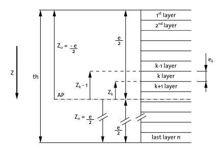
Fig. 2.11 Laminate’s stacking sequence definition and sign convention.

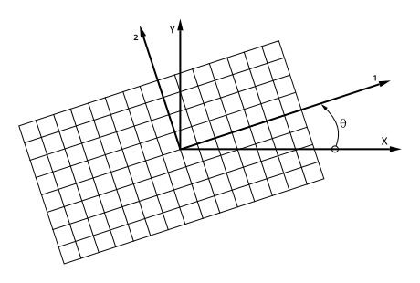
Fig. 2.12 Orientation of individual ply local axes (1,2) in relation to the laminate global axes (x,y).

The basis of the first-order shear deformation theory (FSDT) of plates is given by the following equations:

(2.65)\[\begin{aligned} \varepsilon_x^0 (x,y) = \frac{\partial u_0}{\partial x} \end{aligned}\]

(2.66)\[\begin{aligned} \varepsilon_y^0 (x,y) = \frac{\partial v_0}{\partial y} \end{aligned}\]

(2.67)\[\begin{aligned} \gamma_{xy} (x,y) = \frac{\partial u_0}{\partial y} + \frac{\partial v_0}{\partial x} \end{aligned}\]

(2.68)\[\begin{aligned} \kappa_x (x,y) = \frac{\partial \varPhi_x}{\partial x} \end{aligned}\]

(2.69)\[\begin{aligned} \kappa_y (x,y) = \frac{\partial \varPhi_y}{\partial y} \end{aligned}\]

(2.70)\[\begin{aligned} \kappa_{xy} (x,y) = \frac{\partial \varPhi_x}{\partial y} + \frac{\partial \varPhi_y}{\partial x} \end{aligned}\]

(2.71)\[\begin{aligned} \gamma_{yz} (x,y,z) = - \varPhi_y + \partial w / \partial y \end{aligned}\]

(2.72)\[\begin{aligned} \gamma_{xz} (x,y,z) = - \varPhi_x + \partial w / \partial x \end{aligned}\]

On the other hand, the basis for the classical plate theory (CPT) is given by the following set of equations, where transverse shear deformations (\(\gamma_{yz}\) and \(\gamma_{xz}\)) are neglected:

(2.73)\[\begin{aligned} \varepsilon_x^0 (x,y) = \frac{\partial u_0}{\partial x} \end{aligned}\]

(2.74)\[\begin{aligned} \varepsilon_y^0 (x,y) = \frac{\partial v_0}{\partial y} \end{aligned}\]

(2.75)\[\begin{aligned} \gamma_{xy} (x,y) = \frac{\partial u_0}{\partial y} + \frac{\partial v_0}{\partial x} \end{aligned}\]

(2.76)\[\begin{aligned} \kappa_x (x,y) = \frac{\partial^2 \omega_0}{\partial x^2} \end{aligned}\]

(2.77)\[\begin{aligned} \kappa_y (x,y) = \frac{\partial^2 \omega_0}{\partial y^2} \end{aligned}\]

(2.78)\[\begin{aligned} \kappa_{xy} (x,y) =2 \frac{\partial^2 \omega_0}{\partial x \partial y} \end{aligned}\]

FSDT is more accurate specially in the case of laminated composites since these materials have low shear modulus (G<E/10) thus requiring transverse shear deformations to be taken into account. Up to this point, the strains at every point (x,y,z) of the plate have been replaced by the corresponding mid-surface strains (\(\varepsilon_x^0\), \(\varepsilon_y^0\), \(\gamma_{xy}^0\)) and the surface curvatures (\(\kappa_x\), \(\kappa_y\), \(\kappa_{xy}\)):

(2.79)\[\begin{split}\begin{aligned} \begin{bmatrix} \varepsilon_x \\ \varepsilon_y \\ \gamma_{xy} \end{bmatrix} = \begin{bmatrix} \varepsilon_x^0 \\ \varepsilon_y^0 \\ \gamma_{xy}^0 \end{bmatrix} - z \begin{bmatrix} \kappa_x \\ \kappa_y \\ \kappa_{xy} \end{bmatrix} \end{aligned}\end{split}\]

Integrating the stresses over the thickness of the plate it is possible to obtain the resultant forces and moments per unit width of laminate as:

(2.80)\[\begin{split}\begin{aligned} \begin{bmatrix} N_x \\ N_y \\ N_{xy} \end{bmatrix} = \int_{-\frac{h}{2}}^{\frac{h}{2}} \begin{bmatrix} \sigma_x \\ \sigma_y \\ \tau_{xy} \end{bmatrix} dz \end{aligned}\end{split}\]

(2.81)\[\begin{split}\begin{aligned} \begin{bmatrix} V_x \\ V_y \end{bmatrix} = \int_{-\frac{h}{2}}^{\frac{h}{2}} \begin{bmatrix} \tau_{yz} \\ \tau_{xz} \end{bmatrix} dz \end{aligned}\end{split}\]

(2.82)\[\begin{split}\begin{aligned} \begin{bmatrix} M_x \\ M_y \\ M_{xy} \end{bmatrix} = - \int_{-\frac{h}{2}}^{\frac{h}{2}} \begin{bmatrix} \sigma_x \\ \sigma_y \\ \tau_{xy} \end{bmatrix} \cdot z \, dz \end{aligned}\end{split}\]

Note that with this definition, the moment is positive when the stress is compressive above the mid-surface and tensile below it. Also, positive curvature results in a deflection \(\omega(x,y)\) that is concave up, as it happens in a simply supported beam under its own weight.

For a laminate, the above defined integrals span over several plies. Therefore, the integrals can be divided into summations of integrals over each lamina.

The laminate stiffness matrix can be defined as follows:

(2.83)\[\begin{split}\begin{aligned} \begin{bmatrix} \boldsymbol{N} \\ \boldsymbol{M} \end{bmatrix}_L = \begin{bmatrix} \boldsymbol{A} & \boldsymbol{B} \\ \boldsymbol{B} & \boldsymbol{D} \end{bmatrix}_L : \begin{bmatrix} \varepsilon_{mp} \\ \kappa_{mp} \end{bmatrix}_L \end{aligned}\end{split}\]

(2.84)\[\begin{aligned} \begin{bmatrix} \boldsymbol{V} \end{bmatrix}_L = \begin{bmatrix} \boldsymbol{H} \end{bmatrix}_L : \begin{bmatrix} \gamma_{mp} \end{bmatrix}_L \end{aligned}\]

Where:

(2.85)\[\begin{aligned} \begin{bmatrix} A \end{bmatrix} = \sum_1^n \begin{bmatrix} Q_{ij} \end{bmatrix}_k t_k \quad i,j = 1,2,6 \end{aligned}\]

(2.86)\[\begin{aligned} \begin{bmatrix} B \end{bmatrix} = \sum_1^n \begin{bmatrix} Q_{ij} \end{bmatrix}_k t_k z_k \quad i,j = 1,2,6 \end{aligned}\]

(2.87)\[\begin{aligned} \begin{bmatrix} D \end{bmatrix} = \sum_1^n \begin{bmatrix} Q_{ij} \end{bmatrix}_k \left(t_k z_k^2 + \frac{t_k^3}{12} \right) \quad i,j = 1,2,6 \end{aligned}\]

(2.88)\[\begin{aligned} \begin{bmatrix} H \end{bmatrix} = - \frac{5}{4} \sum_1^n \begin{bmatrix} Q_{ij} \end{bmatrix}_k \left( t_k - \frac{4}{t^2} \left(t_k z_k^2 + \frac{t_k^3}{12}\right) \right) \quad i,j = 4,5 \end{aligned}\]

Note that \(\begin{bmatrix} A \end{bmatrix}\), \(\begin{bmatrix} B \end{bmatrix}\), \(\begin{bmatrix} D \end{bmatrix}\) are all 3x3 symmetric matrices, whose coefficients are functions of the thickness, orientation, stacking sequence, and material properties of the plies [Barbero_2018]. \(\begin{bmatrix} A \end{bmatrix}\) is the in-plane stiffness matrix that relates in-plane strains (\(\varepsilon_x^0\), \(\varepsilon_y^0\), \(\gamma_{xy}^0\)) to in-plane forces (\(N_x\), \(N_y\), \(N_{xy}\)). \(\begin{bmatrix} D \end{bmatrix}\) is the bending stiffness matrix that relates curvatures (\(\kappa_x\), \(\kappa_y\), \(\kappa_{xy}\)) to bending moments (\(M_x\), \(M_y\), \(M_{xy}\)). \(\begin{bmatrix} B \end{bmatrix}\) is the bending-extension coupling matrix that relates the in-plane strains to the bending moments and curvatures to in-plane forces. And finally, \(\begin{bmatrix} H \end{bmatrix}\) is the transverse shear stiffness matrix that relates transverse shear strains (\(\tau_{yz}\), \(\tau_{xz}\)) to transverse shear forces (\(V_x\), \(V_y\)). The bending effect accounted for by \(\begin{bmatrix} B \end{bmatrix}\) does not exist for homogeneous plates. Actually, if the laminate is symmetric with respect to the middle surface, all the bending-extension coupling coefficients \(\begin{bmatrix} B_{ij} \end{bmatrix}\) are zero. On the other hand, matrix \(\begin{bmatrix} H \end{bmatrix}\) is only used within the context of first-order shear deformation theory (FSDT) and not within the classical plate theory (CPT) because in the latter transverse shear strains (\(\tau_{yz}\), \(\tau_{xz}\)) are assumed to be zero.

A set of effective laminate engineering material properties (Young’s modulus, shear modulus and Poisson’s ratios) can be determined from the laminate stiffness matrix, plate thickness and plate bending stiffness of the actual laminate [Barbero_2018].

(2.89)\[\begin{aligned} E_x = \frac{A_{11} A_{22} - A_{12}^2}{t \cdot A_{22}} \end{aligned}\]

(2.90)\[\begin{aligned} E_y = \frac{A_{11} A_{22} - A_{12}^2}{t \cdot A_{11}} \end{aligned}\]

(2.91)\[\begin{aligned} \nu_{xy} = \frac{A_{12}}{A_{22}} \end{aligned}\]

(2.92)\[\begin{aligned} G_{xy} = \frac{A_{66}}{t} \end{aligned}\]

(2.93)\[\begin{aligned} G_{yz} = \frac{H_{44}}{t} \end{aligned}\]

(2.94)\[\begin{aligned} G_{xz} = \frac{H_{55}}{t} \end{aligned}\]

Summarizing, the Classical Lamination Theory uses the ply unidirectional data, ply thickness, orientation and stacking sequence of the plies to determine the laminate stiffness matrix. The ply modulus matrix is determined from the unidirectional properties for each ply. The stress and strain transformation matrices are determined for each ply and used to transform the modulus terms to the laminate reference axis. Next section is devoted to explain how individual ply elastic properties can be obtained from the actual properties of the composite material components (i.e. fibre and matrix).

2.1.4.1.3. Lamina equivalent elastic properties

Table 2.4 Glossary

Symbol	Description	SI units
\(E_{f0^\circ}\)	Longitudinal Young modulus of fibre	\(N/mm2\)
\(E_{f90^\circ}\)	Transverse Young modulus of fibre	\(N/mm2\)
\(E_m\)	Young modulus of the matrix	\(N/mm2\)
\(G_f\)	Shear modulus of the fibre	\(N/mm2\)
\(G_m\)	Shear modulus of the matrix	\(N/mm2\)
\(V_f\)	Volume fraction of fibre in an individual ply	\(-\)
\(\nu_f\)	Fibre’s Poisson coefficient	\(-\)
\(\nu_m\)	Matrix Poisson coefficient	\(-\)
\(E_{UD1}\)	Longitudinal Young’s modulus of an unidirectional ply	\(Pa\)
\(E_{UD2},E_{UD3}\)	Transverse Young’s modulus of an unidirectional ply	\(Pa\)
\(G_{UDij}\)	Shear moduli of an unidirectional ply	\(Pa\)
\(\nu_{UDij}\)	Poisson coefficients for an unidirectional ply	\(-\)
\(e\)	Individual layer thickness	\(m\)
\(C_{eq}\)	Woven balance coefficient for woven roving plies	\(-\)
\(E_{T1}\)	Young modulus in warp direction of a woven roving lamina	\(Pa\)
\(E_{T2}\)	Young modulus in weft direction of a woven roving lamina	\(Pa\)
\(E_{T3}\)	Out-of-plane Young modulus of a woven roving lamina	\(Pa\)
\(G_{Tij}\)	Shear moduli of a woven roving lamina	\(Pa\)
\(\nu_{Tij}\)	Poisson coefficients of a woven roving lamina	\(-\)
\(E_{mat1},E_{mat2}\)	In-plane Young modulus for a strand mat lamina	\(Pa\)
\(E_{mat3}\)	Out-of-plane Young modulus for a strand mat lamina	\(Pa\)
\(G_{mat,ij}\)	Shear modulus of a strand mat lamina	\(Pa\)
\(\nu_{mat,ij}\)	Poisson coefficients of a strand mat lamina	\(-\)

In this section, expressions are presented that can be used to obtain the elastic properties of individual plies from the actual properties of their constituent materials. The formulation presented is in accordance with that reported in [NR546].

The elastic properties of an unidirectional (UD) lamina are estimated from the properties of its constituents as follows:

(2.95)\[\begin{aligned} E_{UD1}=C_{UD1} \cdot \left(E_{f0^\circ} \cdot V_f+E_m \cdot V_m \right) \end{aligned}\]

(2.96)\[\begin{aligned} E_{UD2} = E_{UD3} = C_{UD2} \cdot \left( \frac{E_m}{1-V_m^2} \cdot \frac{1+0.85 \cdot V_f^2}{(1-V_f^2)^{1.25} + \frac{E_m}{E_{f0^\circ}} \cdot \frac{V_f}{1-V_m^2}} \right) \end{aligned}\]

(2.97)\[\begin{aligned} G_{UD12} = G_{UD13} = C_{UD2} \cdot G_m \cdot \frac{1+\eta V_f}{1-\eta V_f} \end{aligned}\]

(2.98)\[\begin{aligned} G_{UD23}=0.7 \cdot G_{UD12} \end{aligned}\]

(2.99)\[\begin{aligned} \eta = \frac{\left(\frac{G_f}{G_m}\right) -1 }{\left(\frac{G_f}{G_m}\right) +1} \end{aligned}\]

(2.100)\[\begin{aligned} \nu_{UD13} = \nu_{UD12} = C_{UD \nu} \cdot \left[\nu_f \cdot V_f + \nu_m \cdot V_m \right] \end{aligned}\]

(2.101)\[\begin{aligned} \nu_{UD21} = \nu_{UD31} = \nu_{UD12} \cdot \frac{E_{UD2}}{E_{UD1}} \end{aligned}\]

(2.102)\[\begin{aligned} \nu_{UD32} = \nu_{UD23} = C_{UD\nu} \cdot \left[\nu_f^{'} \cdot V_f + \nu_m \cdot V_m \right] \end{aligned}\]

With

(2.103)\[\begin{aligned} \nu_f^{'} = \nu_f \cdot \frac{E_{f90^\circ}}{E_{f0^\circ}} \end{aligned}\]

In the expressions above, \(C_{UD1}\), \(C_{UD2}\), \(C_{UD12}\) and \(C_{UDν}\) are empirical constants that depend on the actual nature of the fibres being considered. Following reference [BV_2017], actual coefficient values for the most common fibre types are summarized in the following table.

Constant	E_Glass	R_Glass	Carbon HS	Carbon IM	Carbon HM	Para-aramid
\(C_{UD1}\)	1.00	0.09	1.00	0.85	0.90	0.95
\(C_{UD2}\)	0.80	1.20	0.70	0.80	0.85	0.90
\(C_{UD12}\)	0.90	1.20	0.90	0.90	1.00	0.55
\(C_{UD\nu}\)	0.90	0.90	0.80	0.75	0.70	0.90

The elastic properties of for a woven roving lamina are estimated from the properties of its constituents as follows:

(2.104)\[\begin{aligned} E_{T1} = \frac{1}{e} \cdot \left( A_{11} - \frac{A_{12}^2}{A_{22}}\right) \end{aligned}\]

(2.105)\[\begin{aligned} E_{T2} = \frac{1}{e} \cdot \left( A_{22} - \frac{A_{12}^2}{A_{11}}\right) \end{aligned}\]

(2.106)\[\begin{aligned} E_{T3}=E_{UD3} \end{aligned}\]

(2.107)\[\begin{aligned} G_{T12}=\frac{1}{e} \cdot A_{33} \end{aligned}\]

(2.108)\[\begin{aligned} G_{T13}=G_{T23}=0.9 \cdot G_{T12} \end{aligned}\]

(2.109)\[\begin{aligned} \nu_{T12}=A_{12}/A_{22} \end{aligned}\]

(2.110)\[\begin{aligned} \nu_{T21} = \nu_{T12} \cdot \frac{E_{T2}}{E_{T1}} \end{aligned}\]

(2.111)\[\begin{aligned} \nu_{T32}=\nu_{T31}=\frac{\nu_{UD32}+\nu_{UD31}}{2} \end{aligned}\]

(2.112)\[\begin{aligned} \nu_{T13} = \frac{\nu_{UD23} + \nu_{UD13}}{2} \end{aligned}\]

Where:

(2.113)\[\begin{aligned} A_{11} = e \cdot \left[ C_{eq} \cdot Q_{11} + \left( 1-C_{eq} \right) \cdot Q_{22} \right] \end{aligned}\]

(2.114)\[\begin{aligned} A_{12}=e \cdot Q_{12} \end{aligned}\]

(2.115)\[\begin{aligned} A_{33}=e \cdot Q_{33} \end{aligned}\]

(2.116)\[\begin{aligned} Q_{11} = \frac{E_{UD1}}{1- \nu_{UD12} \nu_{UD21}} \end{aligned}\]

(2.117)\[\begin{aligned} Q_{22} = \frac{E_{UD2}}{1- \nu_{UD12} \nu_{UD21}} \end{aligned}\]

(2.118)\[\begin{aligned} Q_{12} = \frac{\nu_{UD21} \cdot E_{UD1}}{1- \nu_{UD12} \nu_{UD21}} \end{aligned}\]

(2.119)\[\begin{aligned} Q_{33} = G_{UD12} \end{aligned}\]

Finally, the elastic properties of a strand mat lamina are estimated from the properties of its constituents as follows:

(2.120)\[\begin{aligned} E_{mat1} = E_{mat2} = \frac{3}{8} \cdot E_{UD1} + \frac{5}{8} \cdot E_{UD2} \end{aligned}\]

(2.121)\[\begin{aligned} E_{mat3} = E_{UD3} \end{aligned}\]

(2.122)\[\begin{aligned} G_{mat12} = \frac{E_{mat1}}{2 \cdot \left(1+\nu_{mat21} \right)} \end{aligned}\]

(2.123)\[\begin{aligned} G_{mat23} = G_{mat31} = 0.7 \cdot G_{UD12} \end{aligned}\]

(2.124)\[\begin{aligned} \nu_{mat12} = \nu_{mat21} = \nu_{mat32} = \nu_{mat13} = 0.3 \end{aligned}\]

2.1.4.1.4. The Tsai-Wu failure criteria

Of the many failure criteria available, RamSeries implements the Tsai-Wu. This corresponds to a first ply failure analysis for which the sequence of load application is not significant. First ply failure criteria can be used to assess the global strength of a laminate and is the most common criteria used in linear analysis. Within this context, the structural integrity is usually reported in terms of a reserve factor or margin of safety R. Nevertheless, many of the failure criteria are formulated in terms of an expression that provides a failure index FI, where failure is considered to have occurred if the failure index is equal or greater than unity.

The Tsai Wu failure criteria, like the Hoffman criteria, takes into account the difference in tensile and compressive strengths in the longitudinal and transverse directions of the ply. The failure index is given by [Hopkins_2005b]:

(2.125)\[\begin{aligned} FI = F_{11} \sigma_1^2 + F_{22} \sigma_2^2 + 2 F_{12} (\sigma_1 \sigma_2) + F_{66} \sigma_{12}^2 + F_1 \sigma_1 + F_2 \sigma_2 \end{aligned}\]

Where

(2.126)\[\begin{aligned} F_1 = \frac{1}{S_{t1}} - \frac{1}{S_{c1}} \qquad F_2 = \frac{1}{S_{t2}} - \frac{1}{S_{c2}} \end{aligned}\]

(2.127)\[\begin{aligned} F_{11} = \frac{1}{S_{t1}S_{c1}} \qquad F_{22} = \frac{1}{S_{t2}S_{c2}} \end{aligned}\]

(2.128)\[\begin{aligned} F_{66} = 1/T_{12}^2 \qquad F_{12} = -0.5 (F_{11} F_{22})^{0.5} \end{aligned}\]

By replacing the applied stress by the strength (defined as a ratio R times the applied stress) in the failure index expression, Eq. (2.125), and equating to unity the following expression is obtained:

(2.129)\[\begin{aligned} 1.0 = F_{11} R^2 \sigma_1^2 + F_{22} R^2 \sigma_2^2 + 2 F_{12} R^2 (\sigma_1 \sigma_2) + F_{66} R^2 \sigma_{12}^2 + F_1 R \sigma_1 + F_2 R \sigma_2 \end{aligned}\]

The strength ratio \(R\) can be seen as a safety factor or reserve factor, so that if \(R>1\) the applied stress level is below the strength of the material. On the other hand, if \(R<1\) then failure is predicted.

The above expression can be arranged in quadratic form as:

(2.130)\[\begin{aligned} a R^2 + b R + c = 0 \end{aligned}\]

Where

(2.131)\[\begin{aligned} a=[F_{11} \sigma_1^2 + F_{22} \sigma_2^2 + 2 F_{12} (\sigma_1 \sigma_2) + F_{66} \sigma_{12}^2] \end{aligned}\]

(2.132)\[\begin{aligned} b=[F_1 R \sigma_1 + F_2 R \sigma_2] \end{aligned}\]

(2.133)\[\begin{aligned} c=-1.0 \end{aligned}\]

By solving for R, the reserve factor \(R_F\) is obtained.